我在了解高斯过程拟合的过程中,在 brms 包[1]的 gp() 函数帮助文档中发现 mgcv 包[2]的 gamSim() 函数,这个函数打包了一些数据模拟的过程,这个具体过程需要看该函数的源代码。
1 模拟一组数据
举个具体的例子,用 mgcv 的函数 gamSim() 模拟一个响应变量为泊松分布的可加模型。样本量 n = 400 标准差 scale = .2 响应变量是泊松分布 dist = "poisson" 。
set.seed(2024) # 随机数种子用以可复现
dat <- mgcv::gamSim(eg = 1, n = 400, scale = .2, dist = "poisson")
## Gu & Wahba 4 term additive model
head(dat)
##    y     x0      x1     x2       x3      f     f0    f1        f2 f3
## 1  2 0.8369 0.50087 0.9773 0.004902 0.7407 0.9803 2.723 0.0000214  0
## 2 31 0.3209 0.88600 0.1769 0.053554 3.0951 1.6916 5.883 7.9014847  0
## 3  5 0.6804 0.68274 0.7848 0.901255 1.3977 1.6874 3.918 1.3833680  0
## 4 41 0.6982 0.98906 0.2207 0.699616 3.5475 1.6248 7.229 8.8835691  0
## 5  3 0.4570 0.21836 0.5753 0.726998 1.3149 1.9818 1.548 3.0449534  0
## 6  1 0.7014 0.05555 0.5531 0.833525 1.1258 1.6128 1.118 2.8988436  0
随机变量 \(x_0,x_1,x_2,x_3\) 都是服从区间 \([0,1]\) 的均匀分布。f 是 \(f_0,f_1,f_2,f_3\) 的和。gamSim() 函数所用示例修改自文献 [3] 。
\[ \begin{aligned} f_0 &= 2 \sin(\pi x) \\ f_1 &= \exp(2x) \\ f_2 &= 0.2 \times 10^6 x^{11}(1 - x)^6 + 10^4 x^3 (1 - x)^{10} \\ f_3 &= 0 x \end{aligned} \]
\(f_0\) 正弦函数,\(f_1\) 指数函数,\(f_2\) 高阶多项式函数,\(f_3\) 常数函数。四个函数 \(f_0,f_1,f_2,f_3\) 的图像见下图。
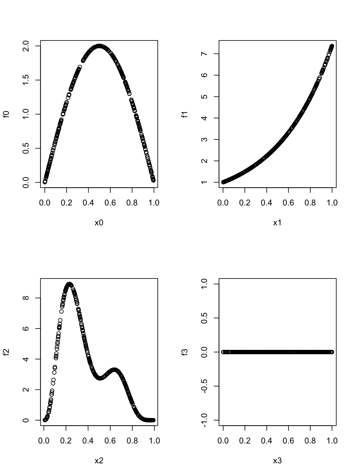
图 1.1: 四个函数 \(f_0,f_1,f_2,f_3\) 的图像
2 广义可加模型
mgcv 包的函数 gam() 专门用来拟合广义可加模型,该 R 包有 20 多年的开发维护历史,已是 R 软件内置的扩展包。
library(mgcv)
## Loading required package: nlme
## This is mgcv 1.9-1. For overview type 'help("mgcv-package")'.
# 拟合数据
fit_gam <- gam(y ~ s(x0, bs = "cr") + s(x1, bs = "cr") + s(x2, bs = "cr") + s(x3, bs = "cr"),
  family = poisson, data = dat, method = "REML"
)
mgcv 包的样条函数 s() 设置 s(bs = "cr") 表示立方样条。
# 模型输出
summary(fit_gam)
##
## Family: poisson
## Link function: log
##
## Formula:
## y ~ s(x0, bs = "cr") + s(x1, bs = "cr") + s(x2, bs = "cr") +
## s(x3, bs = "cr")
##
## Parametric coefficients:
## Estimate Std. Error z value Pr(>|z|)
## (Intercept) 1.5551 0.0251 61.9 <2e-16 ***
## ---
## Signif. codes: 0 '***' 0.001 '**' 0.01 '*' 0.05 '.' 0.1 ' ' 1
##
## Approximate significance of smooth terms:
## edf Ref.df Chi.sq p-value
## s(x0) 2.95 3.66 18.56 0.00082 ***
## s(x1) 3.35 4.14 345.81 < 2e-16 ***
## s(x2) 7.81 8.61 845.79 < 2e-16 ***
## s(x3) 1.00 1.00 1.86 0.17333
## ---
## Signif. codes: 0 '***' 0.001 '**' 0.01 '*' 0.05 '.' 0.1 ' ' 1
##
## R-sq.(adj) = 0.792 Deviance explained = 75.4%
## -REML = 905.72 Scale est. = 1 n = 400从调整的 \(R^2\) 和模型解释的偏差比例来看,可加模型效果还不错。四个样条成分中 \(s(x_0)\)、\(s(x_1)\)、\(s(x_2)\) 都是显著的,只有 \(s(x_3)\) 不显著,符合预先的设定。s(x2) 样条基数比较大与函数 \(f_2\) 比较复杂也一致。
plot(fit_gam, pages = 1)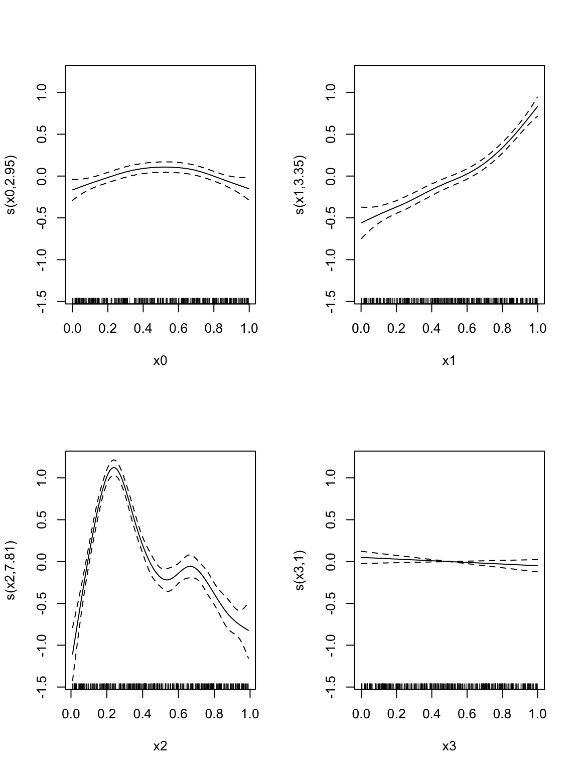
图 2.1: 各个可加项的样条拟合曲线
3 可视化可加模型
下面用 rgl 包和 misc3d 包绘制交互式三维透视图形。rgl 包的 spheres3d() 函数绘制散点图,misc3d 包的 contour3d() 函数绘制等高曲面。
# 设置 Web GL 渲染
options(rgl.useNULL = TRUE)
options(rgl.printRglwidget = TRUE)
# 加载绘图包
library(rgl)
library(misc3d)
# 预测函数
myfun <- function(x, y, z) {
  predict(fit_gam, newdata = data.frame(x0 = x, x1 = y, x2 = z, x3 = 0))
}
# 将数值向量转化为颜色向量
colorize_numeric <- function(x) {
  scales::col_numeric(palette = "Spectral", domain = range(x))(x)
}
# 序列越长对应三维网格密度越大
reso <- 30
# 外加一点缓冲量 10%
limExt <- 0.1
# 各个坐标的范围
ranx <- range(dat$x0)
rany <- range(dat$x1)
ranz <- range(dat$x2)
# 序列化数值向量
xs <- seq(ranx[1] - diff(ranx) * limExt, ranx[2] + diff(ranx) * limExt, length.out = reso)
ys <- seq(rany[1] - diff(rany) * limExt, rany[2] + diff(rany) * limExt, length.out = reso)
zs <- seq(ranz[1] - diff(ranz) * limExt, ranz[2] + diff(ranz) * limExt, length.out = reso)
# 设置等高(值)线/曲面数量
nlevs <- 5
vran <- range(log(dat$y + 1))
levs <- seq(vran[1], vran[2], length.out = nlevs + 2)[-c(1, nlevs + 2)]
# 设置等高(值)线/曲面颜色
levcols <- colorize_numeric(levs)
下面是绘图部分,依此绘制散点、等高线和外框,颜色值根据线性预测生成,响应变量值要取对数(因响应变量服从泊松分布),红色表示值小,蓝色表示值大,为了处理响应变量为 0 的情况,在原值上加 1。
## 绘制散点
with(dat, spheres3d(
  x = x0, y = x1, z = x2,
  col = colorize_numeric(log(y + 1)),
  radius = 0.02
))
## 绘制等高线
contour3d(
  f = myfun,    # 线性预测值
  level = levs, # 等高面的数量
  x = xs, y = ys, z = zs, # 坐标
  color = levcols, # 等高面的颜色
  engine = "rgl", # 渲染引擎
  add = TRUE, # 追加
  alpha = 0.5 # 透明度
)
## 添加外框
box3d()
图 3.1: 可加模型的三维可视化
可加模型的三维可视化
这个等值曲面的形状是非常复杂的,因为广义可加模型的三个成分比较复杂,特别是 \(f_2\) 。
4 运行环境
xfun::session_info(packages = c(
  "mgcv", "rgl", "misc3d"
), dependencies = FALSE)
## R version 4.4.3 (2025-02-28)
## Platform: x86_64-apple-darwin20
## Running under: macOS Sequoia 15.3.2
##
## Locale: en_US.UTF-8 / en_US.UTF-8 / en_US.UTF-8 / C / en_US.UTF-8 / en_US.UTF-8
##
## Package version:
## mgcv_1.9-1 misc3d_0.9-1 rgl_1.3.175 参考文献
主要参考一篇博客 Visualizing model predictions in 3d 。本文所不同者在于去掉了大量的软件依赖,添加了详细的代码注释和模型解释。