1 相关背景
Steven L. Scott 将贝叶斯结构时间序列模型 (Bayesian structural time series,也叫贝叶斯状态空间模型 Bayesian State Space Models)应用在谷歌搜索热度和谷歌分析 Google Analytics中的趋势预测组件中,该模型也被用于推断因果效应(Brodersen et al. 2015),用以评估广告效果。模型的算法理论见论文,本文介绍如何使用他为此开发的 Boom 框架。这个框架很低调,也就他一人在维护,我是在了解 Google Analytics 的预测和异常检测时发现的。
Boom 的扩展包 BoomSpikeSlab 和 bsts 一起实现贝叶斯结构时间序列回归模型(带协变量的),在回归系数上设置 spike-and-slab 先验信息,引入稀疏性,收缩(正则)回归系数,实现变量选择,极大降低回归问题的规模。另有一个类似功能的 R包值得一提,bssm 包也是基于贝叶斯方法拟合状态空间模型,使用的 MCMC 采样算法是自适应随机游走 Metropolis 算法和 particle filters 算法。
2 准备工作
先加载几个 R 包
library(Boom)
library(BoomSpikeSlab)
library(bsts)复用之前一篇文章《大规模时序预测 Prophet》的示例数据—佩顿·曼宁的维基百科页面的访问量(的对数)。
# https://xiangyun.rbind.io/2024/05/forecasting-at-scale/data/peyton_manning.csv
# 加载数据
df <- read.csv('../2024-05-01-forecasting-at-scale/data/peyton_manning.csv', colClasses = c("Date", "numeric"))
str(df)
## 'data.frame': 2905 obs. of 2 variables:
## $ ds: Date, format: "2007-12-10" "2007-12-11" ...
## $ y : num 9.59 8.52 8.18 8.07 7.89 ...数据整理,时间序列预测要先观察一下数据中的历史规律,就是关于时间的变化规律,从日期一列扩展出年、周等列,以便后续探索。
df$weekday <- format(df$ds, format = "%a")
df$weekday <- factor(df$weekday, levels = c("Sun", "Mon", "Tue", "Wed", "Thu", "Fri", "Sat"))
df$year <- format(df$ds, format = "%Y")
df$day_of_year <- as.integer(format(df$ds, "%j"))
数据探索,先看每年的变化趋势,再看每周的变化趋势。
library(ggplot2)
ggplot(data = df, aes(x = day_of_year, y = y, color = year)) +
  geom_point()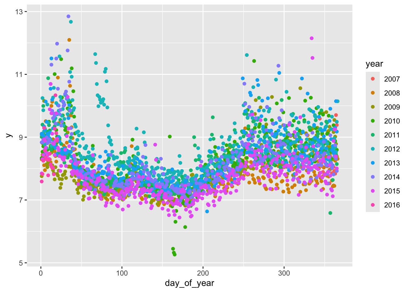
从每年访问量的波动变化来看,有很强的季节性(周期性),波动变化是非线性的。考虑到每年波动情况的季节性,提取一部分数据观察周访问量。
ggplot(data = df[df$year >= 2015,], aes(x = ds, y = y)) +
  geom_point(aes(color = weekday))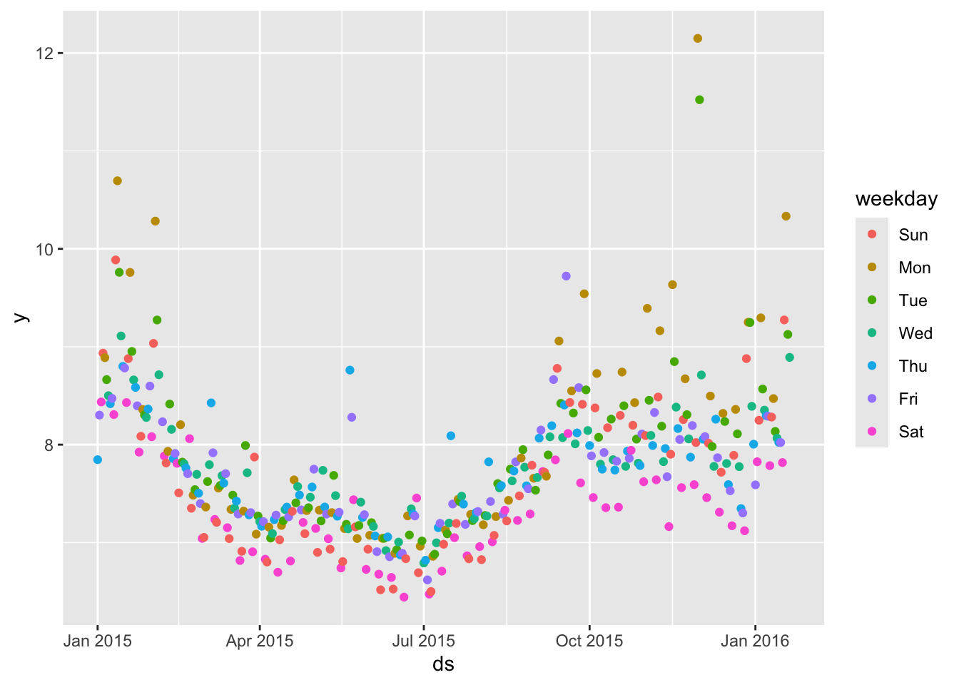
从每周访问量的波动变化来看,也有很强的季节性(周期性),且波动变化也是非线性的。
3 模型拟合
通过上述探索和分析,可以发现数据存在很强的季节性和非线性趋势。
library(bsts)
y = df[df$year>=2013,"y"]
# 局部线性趋势
ss1 <- AddLocalLinearTrend(list(), y)
# 一周 7 天
ss1 <- AddSeasonal(ss1, y, nseasons = 7)
# 拟合模型
model1 <- bsts(y, state.specification = ss1, niter = 500, seed = 2024)
## =-=-=-=-= Iteration 0 Fri May 8 13:34:48 2026 =-=-=-=-=
## =-=-=-=-= Iteration 50 Fri May 8 13:34:48 2026 =-=-=-=-=
## =-=-=-=-= Iteration 100 Fri May 8 13:34:48 2026 =-=-=-=-=
## =-=-=-=-= Iteration 150 Fri May 8 13:34:49 2026 =-=-=-=-=
## =-=-=-=-= Iteration 200 Fri May 8 13:34:49 2026 =-=-=-=-=
## =-=-=-=-= Iteration 250 Fri May 8 13:34:50 2026 =-=-=-=-=
## =-=-=-=-= Iteration 300 Fri May 8 13:34:50 2026 =-=-=-=-=
## =-=-=-=-= Iteration 350 Fri May 8 13:34:51 2026 =-=-=-=-=
## =-=-=-=-= Iteration 400 Fri May 8 13:34:51 2026 =-=-=-=-=
## =-=-=-=-= Iteration 450 Fri May 8 13:34:51 2026 =-=-=-=-=# 可视化拟合
plot(model1)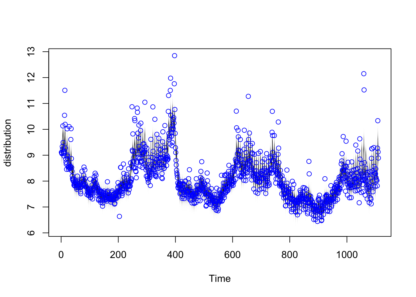
图中蓝色的散点是真实的数据值
# 分别展示趋势和季节性成分
plot(model1, "components")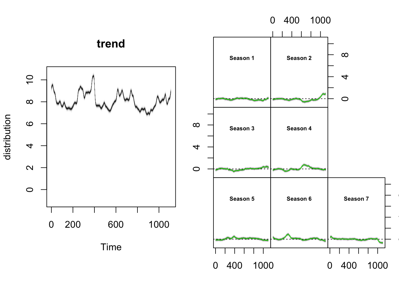
# 拟合的残差的分布
plot(model1, "residuals", burn = 100)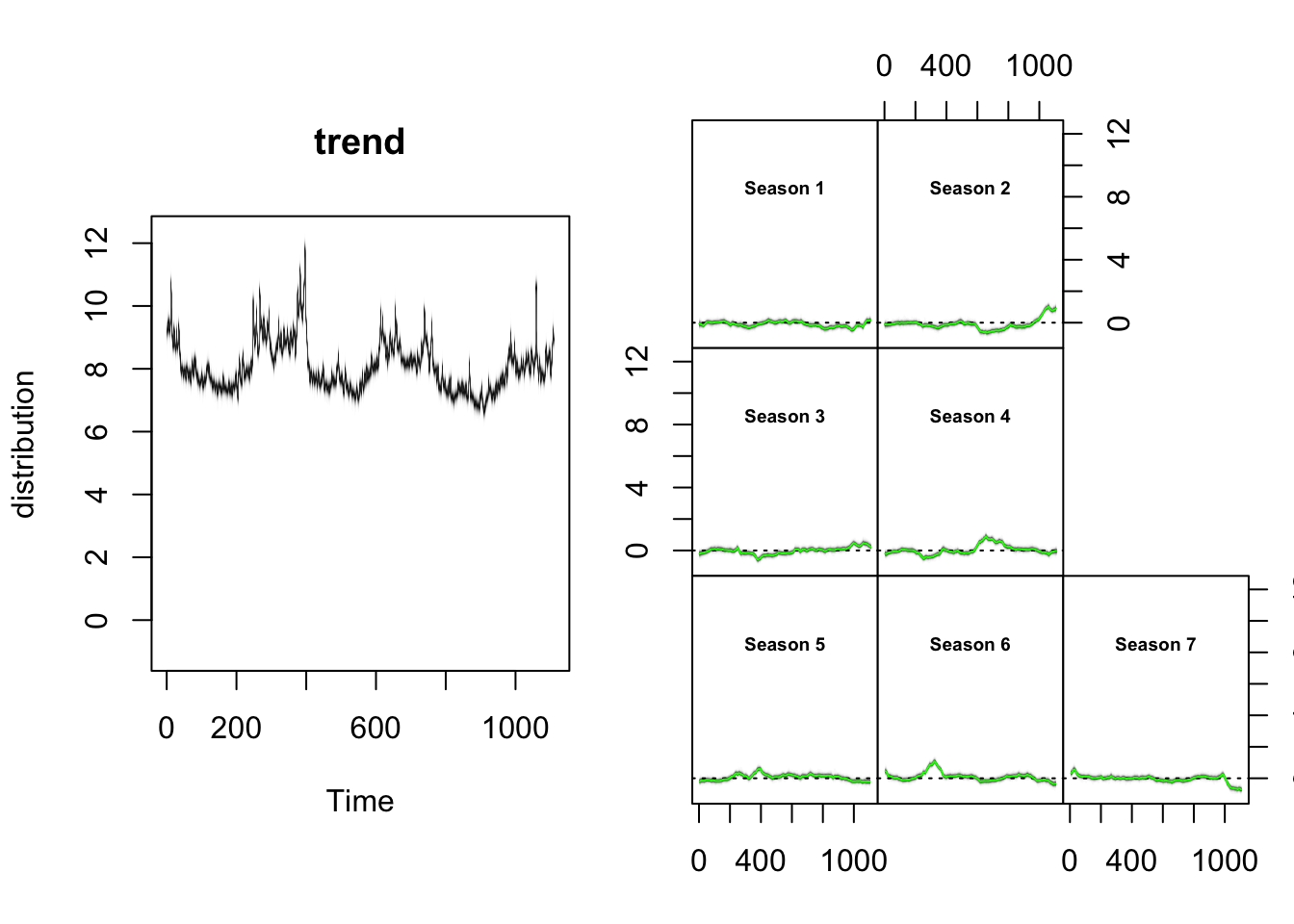
趋势拟合
# 预测 14 天
pred1 <- predict(model1, horizon = 14, burn = 100)
# 可视化预测
plot(pred1)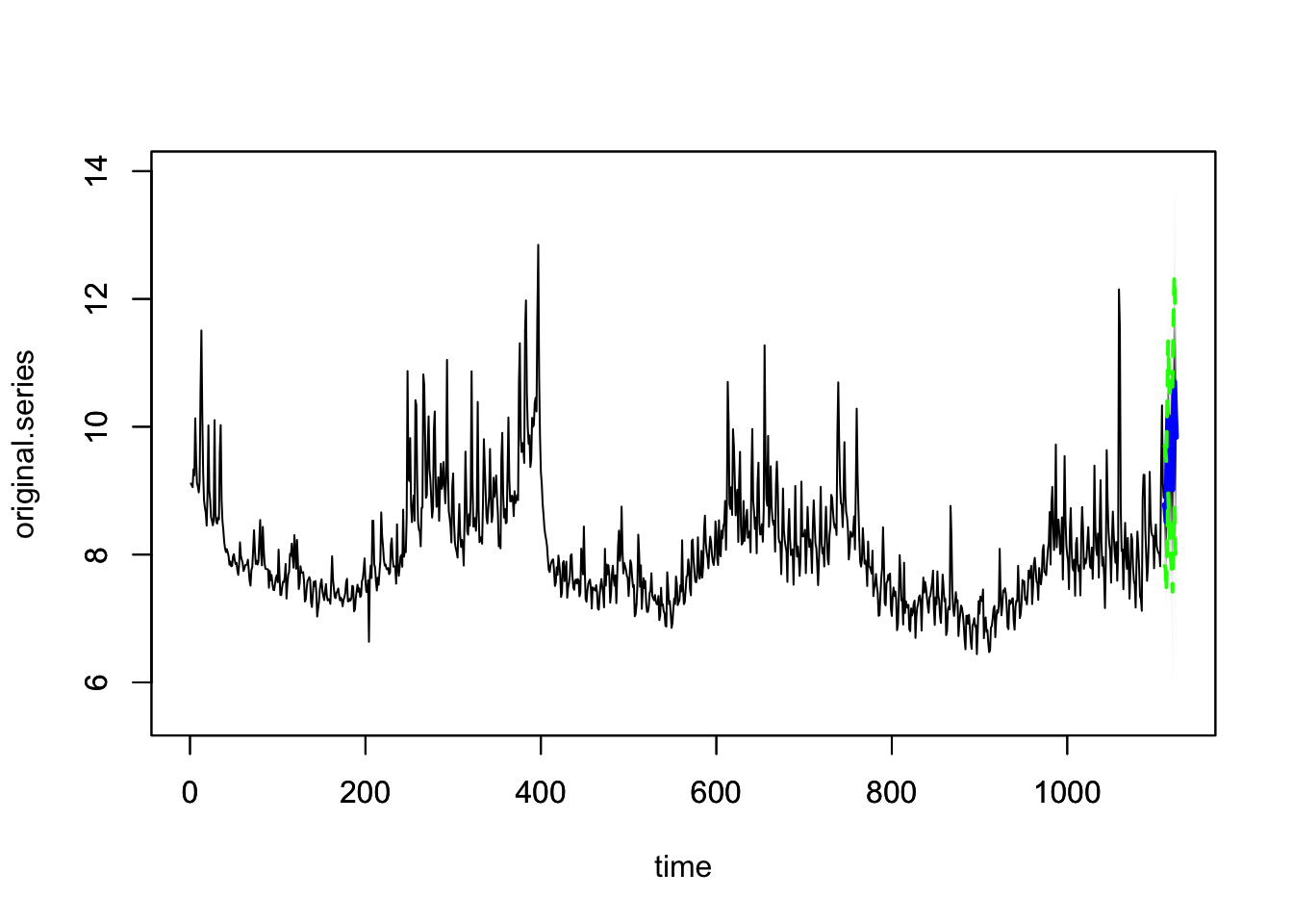
试试半局部线性趋势
ss2 <- AddSemilocalLinearTrend(list(), y)
ss2 <- AddSeasonal(ss2, y, nseasons = 7)
model2 <- bsts(y, state.specification = ss2, niter = 500, seed = 2024)
## =-=-=-=-= Iteration 0 Fri May 8 13:34:55 2026 =-=-=-=-=
## =-=-=-=-= Iteration 50 Fri May 8 13:34:55 2026 =-=-=-=-=
## =-=-=-=-= Iteration 100 Fri May 8 13:34:56 2026 =-=-=-=-=
## =-=-=-=-= Iteration 150 Fri May 8 13:34:56 2026 =-=-=-=-=
## =-=-=-=-= Iteration 200 Fri May 8 13:34:56 2026 =-=-=-=-=
## =-=-=-=-= Iteration 250 Fri May 8 13:34:57 2026 =-=-=-=-=
## =-=-=-=-= Iteration 300 Fri May 8 13:34:57 2026 =-=-=-=-=
## =-=-=-=-= Iteration 350 Fri May 8 13:34:58 2026 =-=-=-=-=
## =-=-=-=-= Iteration 400 Fri May 8 13:34:58 2026 =-=-=-=-=
## =-=-=-=-= Iteration 450 Fri May 8 13:34:58 2026 =-=-=-=-=# 可视化拟合
plot(model2)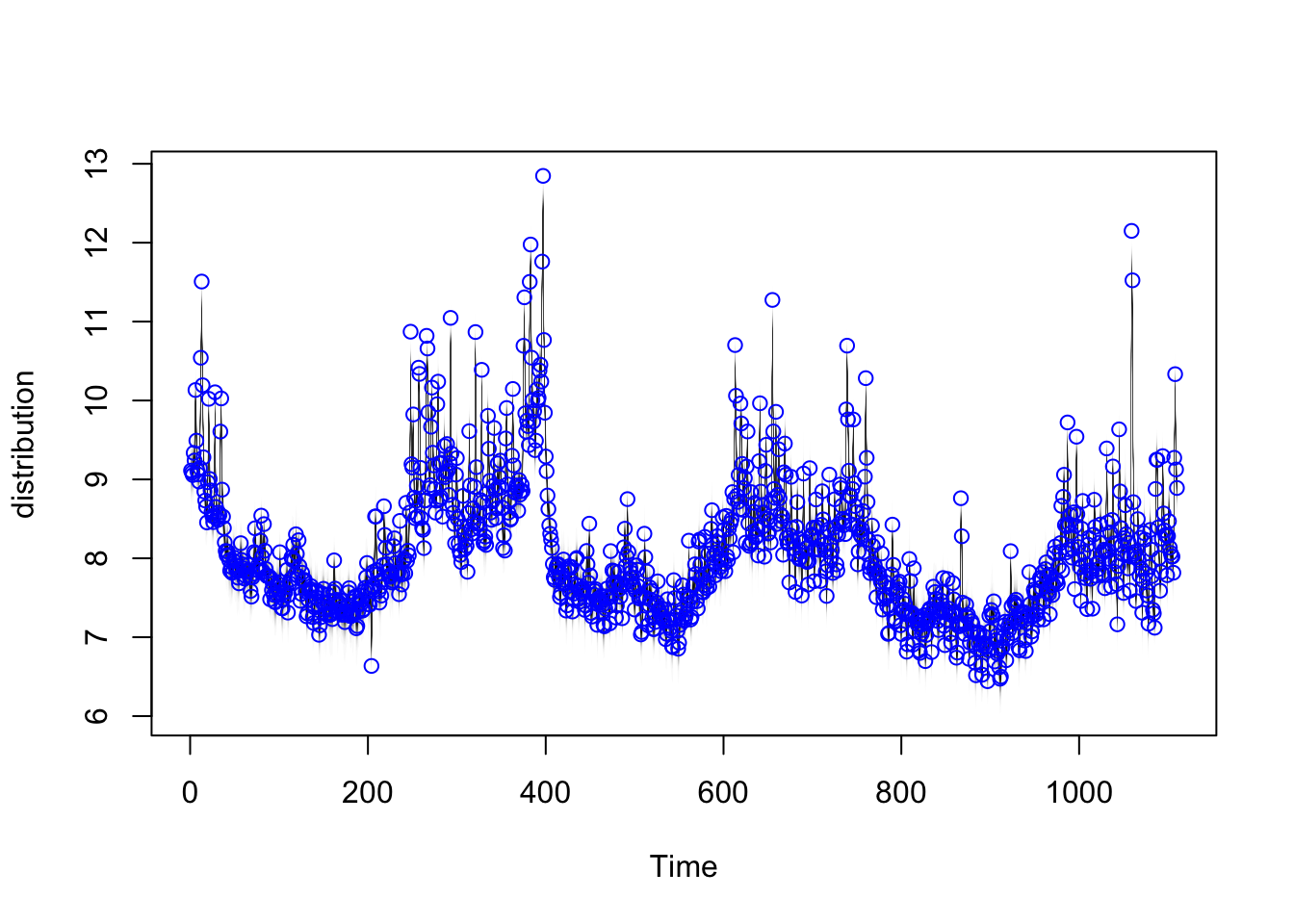
# 分别展示趋势和季节性成分
plot(model2, "components")
# 预测 14 天
pred2 <- predict(model2, horizon = 14, burn = 100)
# 可视化预测
plot(pred2)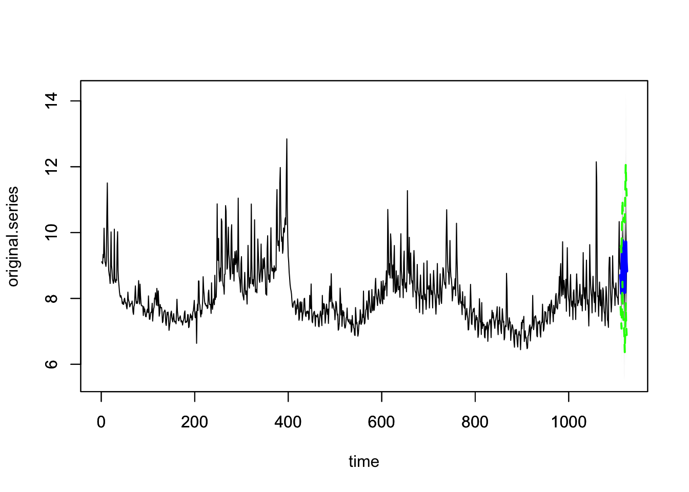
比较预测区间的宽度
range(pred1)## [1] 6.443 13.549range(pred2)## [1] 5.519 14.264选取离预测时间最近的 90 天观测值
# 预测区间较窄更好
plot(pred1, plot.original = 90, ylim = range(pred2))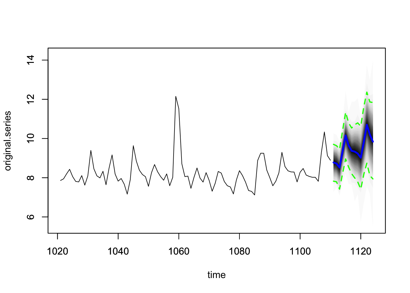
# 预测区间比较宽
plot(pred2, plot.original = 90, ylim = range(pred2))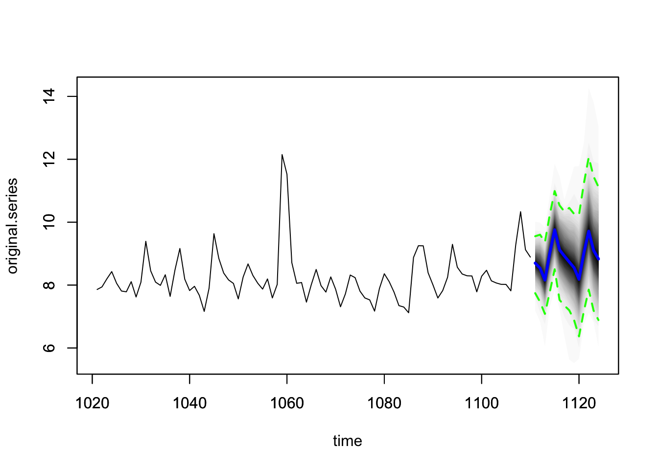
从图上来看,两个模型差别不大。
4 本文总结
Boom、Prophet (Taylor and Letham 2018) 和 INLA 都是贝叶斯模型,Prophet 在工业界比较知名,而 INLA 在学术界比较知名。Prophet 局限于时间序列预测,而 INLA 属于大一统的模型框架。Prophet 基于概率编程语言 Stan ,多采用全贝叶斯精确推断,而 INLA 采用集成嵌套拉普拉斯近似计算。Prophet 需要编译、抽样等过程,速度慢,而 INLA 类似普通 R 包,可以近实时地计算。