用 geopandas 绘制邵阳市各区县的人口分布图

我以前写过 10 篇用 R 语言绘制地图和空间数据可视化相关的博客。

【热门文章】R 语言画中国地图找各种地图数据、检查数据可用性
【热门文章】空间数据可视化与 R 语言（上篇）介绍空间数据操作 sf 包，用 echarts4r、 leaflet、plotly 和 lattice 包绘制可视化图形。
空间数据可视化与 R 语言（中篇）找各类在线地图服务，结合在线地图绘制空间数据的各类可视化图形。
空间数据可视化与 R 语言（下篇）不同类型的空间数据和不同的绘制方法。
【进阶】地区分布图及其应用总结 R 语言中 7 种空间数据可视化的绘图方法。
【进阶】R 语言制作地区分布图及其动画以动画的方式可视化空间数据（时空数据）。
【高阶】预测朗格拉普岛核辐射强度的分布 R 语言做空间分析和建模。
【进阶】中国常住人口分布图（2023 年市级） leaflet 包可视化中国各市的常住人口数及其变化。
地震越来越频繁了吗？ ggplot2 包绘制地图。
highcharter 食谱 highcharter 包绘制地图。

今天，用一些 Python 模块绘制一幅邵阳市人口的空间分布图。

读取邵阳市的地图数据，这是一个 JSON 格式的数据。用 geopandas 模块读取该数据，之后，可以类似 pandas 模块那样操作数据。

import geopandas as gpd
shaoyang = gpd.read_file('data/邵阳市.json')
# 坐标参考系
shaoyang.crs

## <Geographic 2D CRS: EPSG:4326>
## Name: WGS 84
## Axis Info [ellipsoidal]:
## - Lat[north]: Geodetic latitude (degree)
## - Lon[east]: Geodetic longitude (degree)
## Area of Use:
## - name: World.
## - bounds: (-180.0, -90.0, 180.0, 90.0)
## Datum: World Geodetic System 1984 ensemble
## - Ellipsoid: WGS 84
## - Prime Meridian: Greenwich

# 查看前几行数据
shaoyang.head()

##    adcode  ...                                           geometry
## 0  430502  ...  MULTIPOLYGON (((111.60058 27.28676, 111.59138 ...
## 1  430503  ...  MULTIPOLYGON (((111.46854 27.24214, 111.46591 ...
## 2  430511  ...  MULTIPOLYGON (((111.48548 27.2898, 111.47899 2...
## 3  430522  ...  MULTIPOLYGON (((111.82375 27.44738, 111.81949 ...
## 4  430523  ...  MULTIPOLYGON (((111.66976 27.03255, 111.67033 ...
## 
## [5 rows x 10 columns]

显示了行数和列数，第一列和最后一列，中间列的数据都省略了。下面查看行政区域编码 ‘adcode’, 区县名称 ‘name’ 和地理边界 ‘geometry’ 三列。

shaoyang.loc[:, ['adcode', 'name', 'geometry']]

##     adcode     name                                           geometry
## 0   430502      双清区  MULTIPOLYGON (((111.60058 27.28676, 111.59138 ...
## 1   430503      大祥区  MULTIPOLYGON (((111.46854 27.24214, 111.46591 ...
## 2   430511      北塔区  MULTIPOLYGON (((111.48548 27.2898, 111.47899 2...
## 3   430522      新邵县  MULTIPOLYGON (((111.82375 27.44738, 111.81949 ...
## 4   430523      邵阳县  MULTIPOLYGON (((111.66976 27.03255, 111.67033 ...
## 5   430524      隆回县  MULTIPOLYGON (((110.64826 27.36729, 110.65633 ...
## 6   430525      洞口县  MULTIPOLYGON (((110.91961 27.02706, 110.92092 ...
## 7   430527      绥宁县  MULTIPOLYGON (((110.14853 26.9897, 110.14626 2...
## 8   430528      新宁县  MULTIPOLYGON (((110.58552 26.30133, 110.58702 ...
## 9   430529  城步苗族自治县  MULTIPOLYGON (((109.99175 26.26846, 109.99111 ...
## 10  430581      武冈市  MULTIPOLYGON (((110.54002 26.85363, 110.53864 ...
## 11  430582      邵东市  MULTIPOLYGON (((111.60058 27.28676, 111.60498 ...

邵阳市一共 12 个区县。还可以查看所有的列。

# 查看所有的列
shaoyang.columns

## Index(['adcode', 'name', 'center', 'centroid', 'childrenNum', 'level',
##        'parent', 'subFeatureIndex', 'acroutes', 'geometry'],
##       dtype='str')

# 查看所有的列的数据类型
shaoyang.dtypes

## adcode                int32
## name                    str
## center               object
## centroid             object
## childrenNum           int32
## level                   str
## parent               object
## subFeatureIndex       int32
## acroutes             object
## geometry           geometry
## dtype: object

绘制邵阳市区县级行政区划图，默认设置下的效果图。

shaoyang.plot()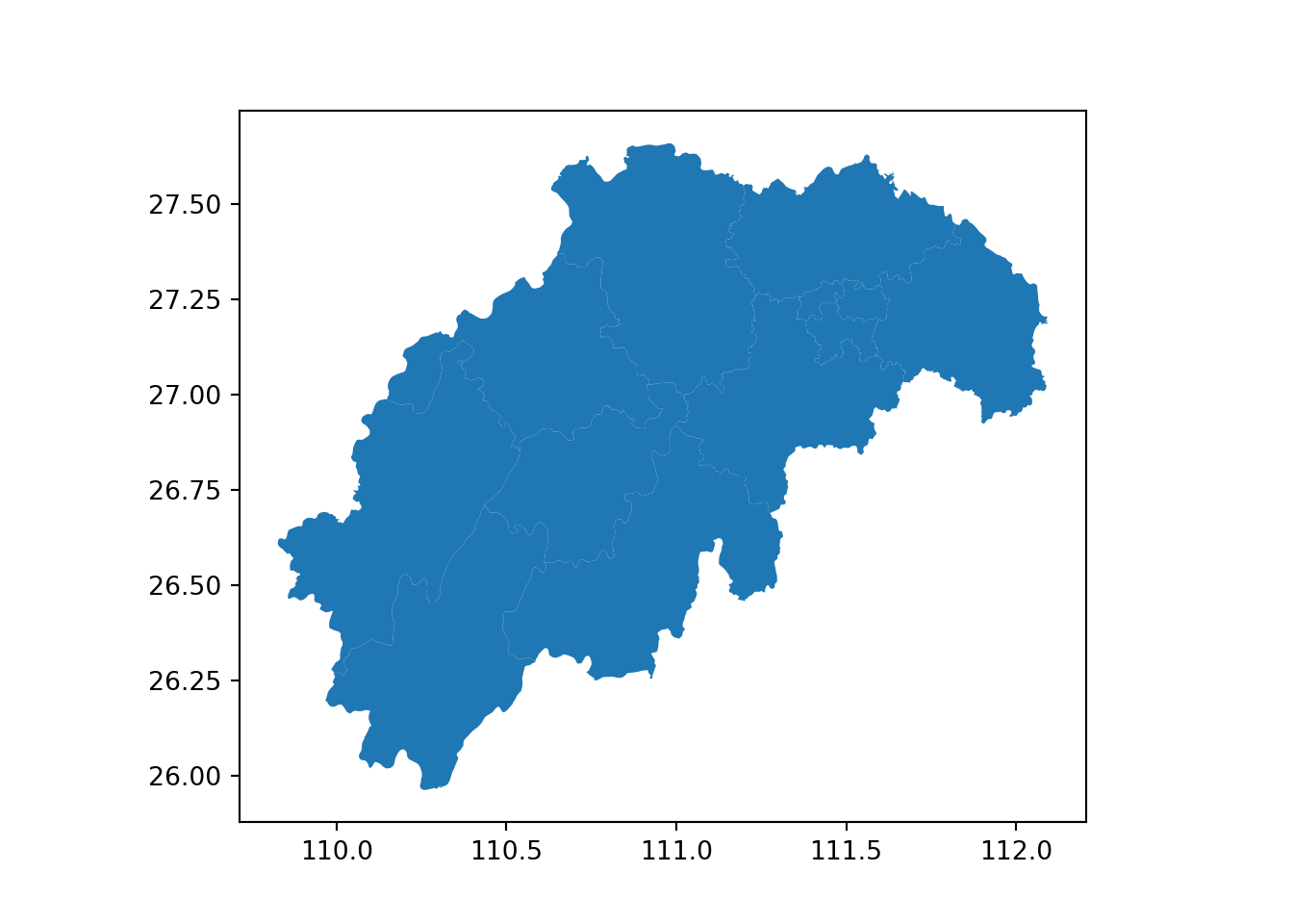

有了地图数据集后，下面准备邵阳市各区县 2023年的常住年末户数（单位：万户）及人口（单位：万人）数据。

import pandas as pd
pop23 = pd.DataFrame(
    {
        "adcode": [430502, 430503, 430511, 430522, 430523, 430524, 430525, 430527, 430528, 430529, 430581, 430582],
        "name": ["双清区", "大祥区", "北塔区", "新邵县", "邵阳县", "隆回县", "洞口县", "绥宁县", "新宁县", "城步苗族自治县", "武冈市", "邵东市"],
        "household": [11.55, 14.14, 4.86, 19.94, 24.01, 35.18, 22.6, 10.83, 16.69, 7.67, 22.65, 36.59],
        "population": [32.01, 36.32, 12.37, 58.59, 71.45, 98.02, 65.71, 28.32, 49.78, 22.11, 62.01, 99.19]
    }
)
pop23

##     adcode     name  household  population
## 0   430502      双清区      11.55       32.01
## 1   430503      大祥区      14.14       36.32
## 2   430511      北塔区       4.86       12.37
## 3   430522      新邵县      19.94       58.59
## 4   430523      邵阳县      24.01       71.45
## 5   430524      隆回县      35.18       98.02
## 6   430525      洞口县      22.60       65.71
## 7   430527      绥宁县      10.83       28.32
## 8   430528      新宁县      16.69       49.78
## 9   430529  城步苗族自治县       7.67       22.11
## 10  430581      武冈市      22.65       62.01
## 11  430582      邵东市      36.59       99.19

调用 pandas 模块的 merge 方法将地图数据和常住人口数据合并至一个数据框内。

mydata = pd.merge(shaoyang.loc[:, ['name', 'geometry']], pop23, on="name")

最后，借助模块 geopandas 的 plot 方法绘制可视化图形，指定要可视化的数据列，选择一个合适的调色板，显示图例。

mydata.plot(column="population", cmap='OrRd', legend=True)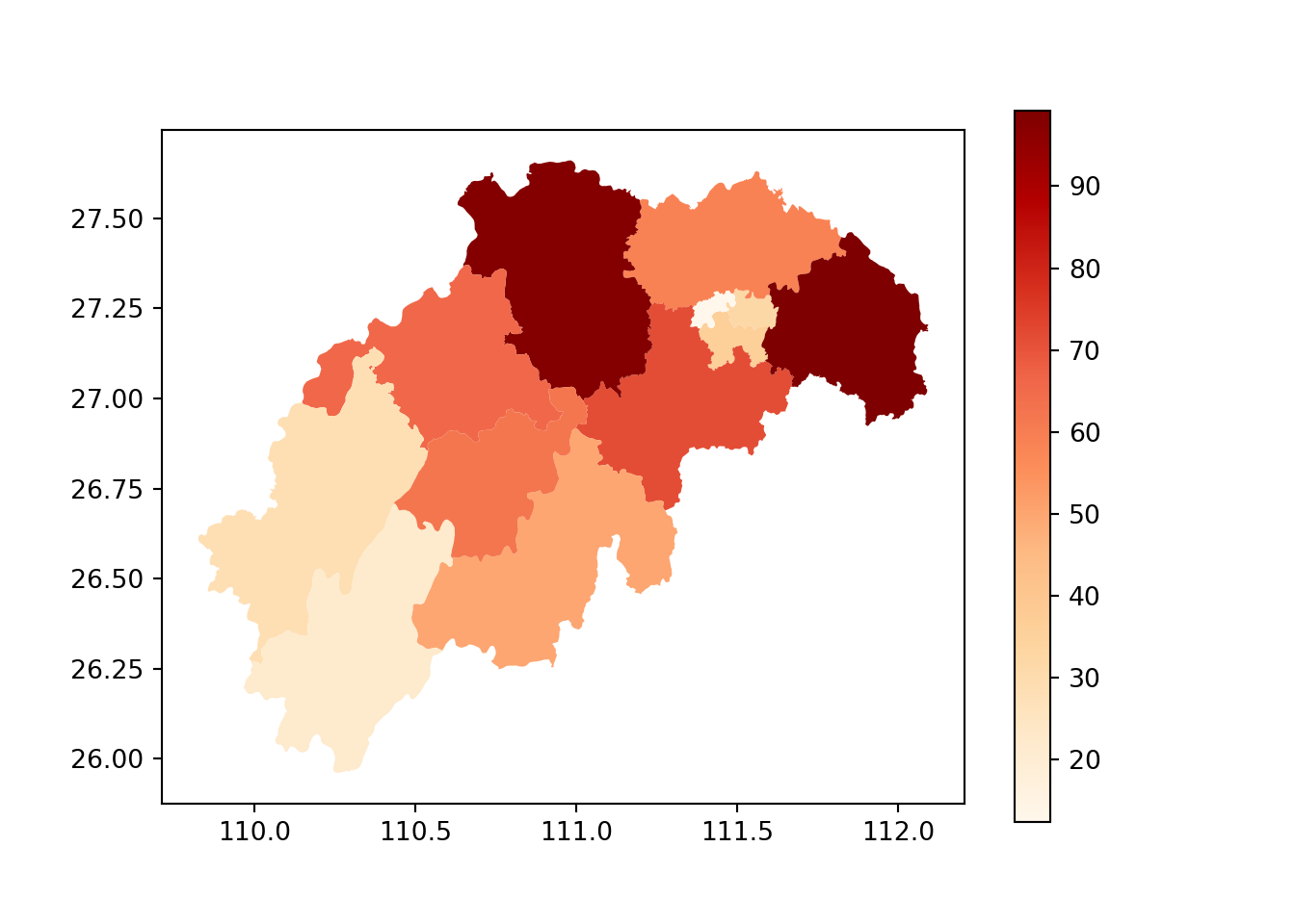

matplotlib 模块内置的调色板还有很多，运行如下代码可查看。

from matplotlib import colormaps
# 多少个调色板
len(list(colormaps))

## 180

# 全部显示出来
df = pd.DataFrame(list(colormaps), columns=list("A"))
df["A"].to_numpy()

## array(['magma', 'inferno', 'plasma', 'viridis', 'cividis', 'twilight',
##        'twilight_shifted', 'turbo', 'berlin', 'managua', 'vanimo',
##        'Blues', 'BrBG', 'BuGn', 'BuPu', 'CMRmap', 'GnBu', 'Greens',
##        'Greys', 'OrRd', 'Oranges', 'PRGn', 'PiYG', 'PuBu', 'PuBuGn',
##        'PuOr', 'PuRd', 'Purples', 'RdBu', 'RdGy', 'RdPu', 'RdYlBu',
##        'RdYlGn', 'Reds', 'Spectral', 'Wistia', 'YlGn', 'YlGnBu', 'YlOrBr',
##        'YlOrRd', 'afmhot', 'autumn', 'binary', 'bone', 'brg', 'bwr',
##        'cool', 'coolwarm', 'copper', 'cubehelix', 'flag', 'gist_earth',
##        'gist_gray', 'gist_heat', 'gist_ncar', 'gist_rainbow',
##        'gist_stern', 'gist_yarg', 'gnuplot', 'gnuplot2', 'gray', 'hot',
##        'hsv', 'jet', 'nipy_spectral', 'ocean', 'pink', 'prism', 'rainbow',
##        'seismic', 'spring', 'summer', 'terrain', 'winter', 'Accent',
##        'Dark2', 'Paired', 'Pastel1', 'Pastel2', 'Set1', 'Set2', 'Set3',
##        'tab10', 'tab20', 'tab20b', 'tab20c', 'grey', 'gist_grey',
##        'gist_yerg', 'Grays', 'magma_r', 'inferno_r', 'plasma_r',
##        'viridis_r', 'cividis_r', 'twilight_r', 'twilight_shifted_r',
##        'turbo_r', 'berlin_r', 'managua_r', 'vanimo_r', 'Blues_r',
##        'BrBG_r', 'BuGn_r', 'BuPu_r', 'CMRmap_r', 'GnBu_r', 'Greens_r',
##        'Greys_r', 'OrRd_r', 'Oranges_r', 'PRGn_r', 'PiYG_r', 'PuBu_r',
##        'PuBuGn_r', 'PuOr_r', 'PuRd_r', 'Purples_r', 'RdBu_r', 'RdGy_r',
##        'RdPu_r', 'RdYlBu_r', 'RdYlGn_r', 'Reds_r', 'Spectral_r',
##        'Wistia_r', 'YlGn_r', 'YlGnBu_r', 'YlOrBr_r', 'YlOrRd_r',
##        'afmhot_r', 'autumn_r', 'binary_r', 'bone_r', 'brg_r', 'bwr_r',
##        'cool_r', 'coolwarm_r', 'copper_r', 'cubehelix_r', 'flag_r',
##        'gist_earth_r', 'gist_gray_r', 'gist_heat_r', 'gist_ncar_r',
##        'gist_rainbow_r', 'gist_stern_r', 'gist_yarg_r', 'gnuplot_r',
##        'gnuplot2_r', 'gray_r', 'hot_r', 'hsv_r', 'jet_r',
##        'nipy_spectral_r', 'ocean_r', 'pink_r', 'prism_r', 'rainbow_r',
##        'seismic_r', 'spring_r', 'summer_r', 'terrain_r', 'winter_r',
##        'Accent_r', 'Dark2_r', 'Paired_r', 'Pastel1_r', 'Pastel2_r',
##        'Set1_r', 'Set2_r', 'Set3_r', 'tab10_r', 'tab20_r', 'tab20b_r',
##        'tab20c_r', 'grey_r', 'gist_grey_r', 'gist_yerg_r', 'Grays_r'],
##       dtype=object)

实际上是 90 个调色板，后缀 _r 表示反向。

geopandas 还可以画各种常规图形，如散点图、折线图、箱线图、直方图。

mydata.plot(kind="scatter", x="household", y="population")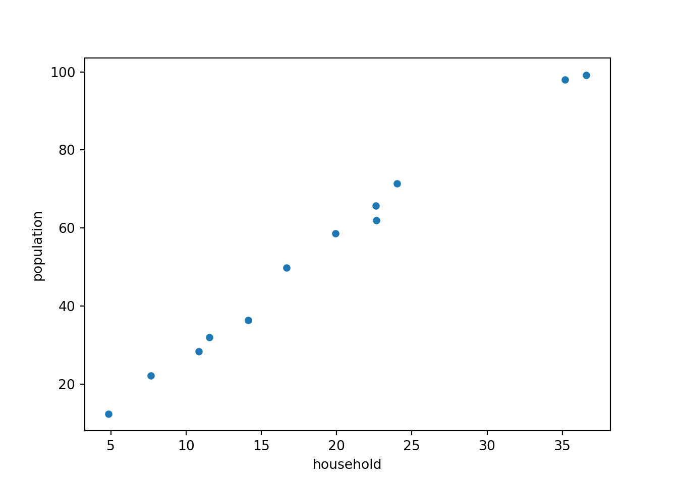

geopandas 还可以绘制交互图形，此时，需要安装额外的 Python 模块 folium （调用 leaflet.js）和 mapclassify 。

mydata.explore(column="population", tooltip="population", cmap='OrRd')

Make this Notebook Trusted to load map: File -> Trust Notebook

下面补充本文运行的环境。

reticulate::py_config()

## python:         /opt/.virtualenvs/r-tensorflow/bin/python
## libpython:      /opt/homebrew/opt/python@3.13/Frameworks/Python.framework/Versions/3.13/lib/python3.13/config-3.13-darwin/libpython3.13.dylib
## pythonhome:     /opt/.virtualenvs/r-tensorflow:/opt/.virtualenvs/r-tensorflow
## virtualenv:     /opt/.virtualenvs/r-tensorflow/bin/activate_this.py
## version:        3.13.11 (main, Dec  5 2025, 16:06:33) [Clang 17.0.0 (clang-1700.4.4.1)]
## numpy:          /opt/.virtualenvs/r-tensorflow/lib/python3.13/site-packages/numpy
## numpy_version:  2.3.4
## 
## NOTE: Python version was forced by RETICULATE_PYTHON_ENV

所用 Python 模块的版本，如下。

matplotlib 3.10.7
pandas 3.0.0
geopandas 1.1.3
shapely 2.1.2
folium 0.20.0
mapclassify 2.10.0

这是用到的几个 Python 模块的官方网站。

https://github.com/geopandas/geopandas
https://github.com/shapely/shapely
https://matplotlib.org/stable/
Scientific Visualization: Python + Matplotlib Nicolas P. Rougier, Bordeaux, November 2021. Matplotlib 高级绘图画廊。

黄湘云