1 坐标系统
基于数据集 gapminder 展示坐标变换在柱状图、条形图、饼图中的作用,首先来看笛卡尔坐标系下的柱状图。
library(ggplot2)
library(scales)
gapminder <- readRDS(file = "data/gapminder-2020.rds")
gapminder_2007 <- gapminder[gapminder$year == 2007, ]
ggplot(gapminder_2007, aes(x = income_level)) +
  geom_bar(stat = "count") +
  theme_classic() +
  labs(x = "收入水平", y = "国家数量")
图 1.1: 笛卡尔坐标系下的柱形图
ggplot(gapminder_2007, aes(x = income_level, y = after_stat(count))) +
  geom_bar(stat = "count") +
  theme_classic() +
  labs(x = "收入水平", y = "国家数量")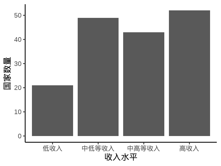
图 1.2: 笛卡尔坐标系下的柱形图
翻转
ggplot(gapminder_2007, aes(x = income_level)) +
  geom_bar(stat = "count") +
  coord_flip() +
  theme_classic() +
  labs(x = "收入水平", y = "国家数量")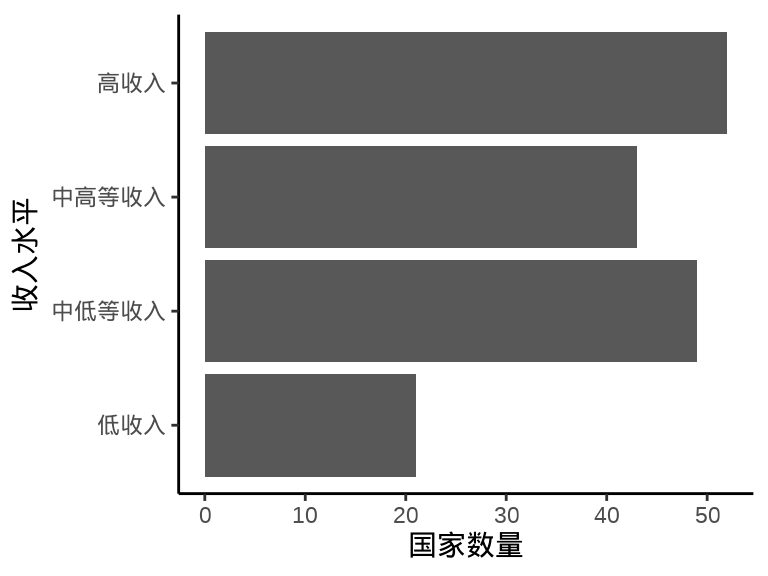
图 1.3: 笛卡尔坐标系下的条形图
极坐标变换
ggplot(gapminder_2007, aes(x = income_level)) +
  geom_bar(stat = "count") +
  coord_polar() +
  theme_minimal() +
  labs(x = NULL, y = NULL)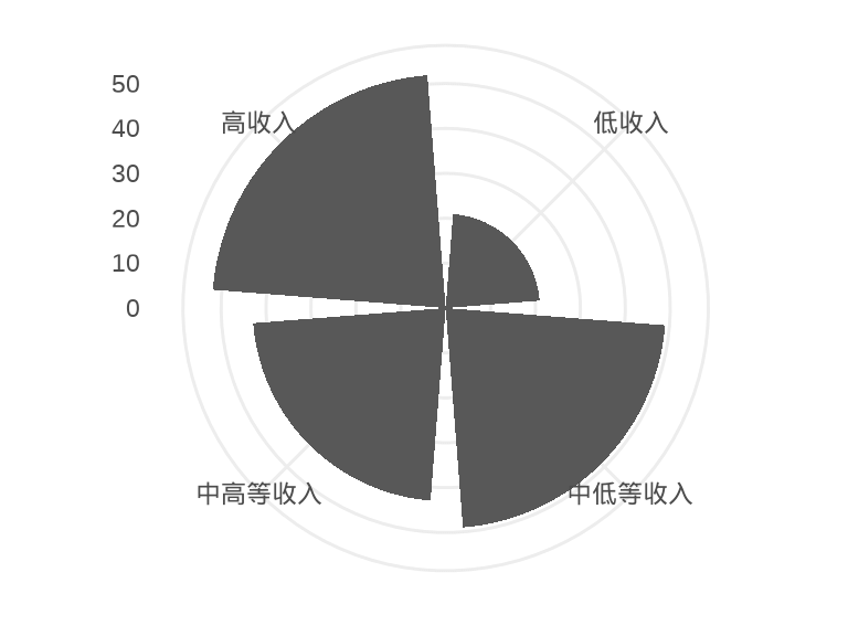
图 1.4: 极坐标系下的条形图
极坐标变换
ggplot(gapminder_2007, aes(x = income_level)) +
  geom_bar(stat = "count") +
  coord_polar(theta = "y") +
  theme_minimal() +
  labs(x = NULL, y = NULL)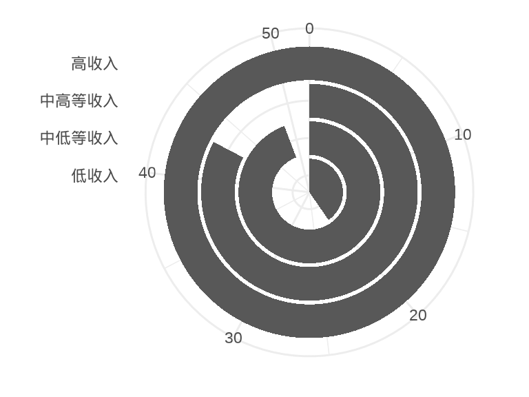
图 1.5: 极坐标系下的柱形图
笛卡尔坐标系下的分组堆积柱形图
ggplot(gapminder_2007, aes(x = income_level, fill = region)) +
  geom_bar(stat = "count") +
  theme_classic() +
  labs(x = "收入水平", y = "国家数量", fill = "区域")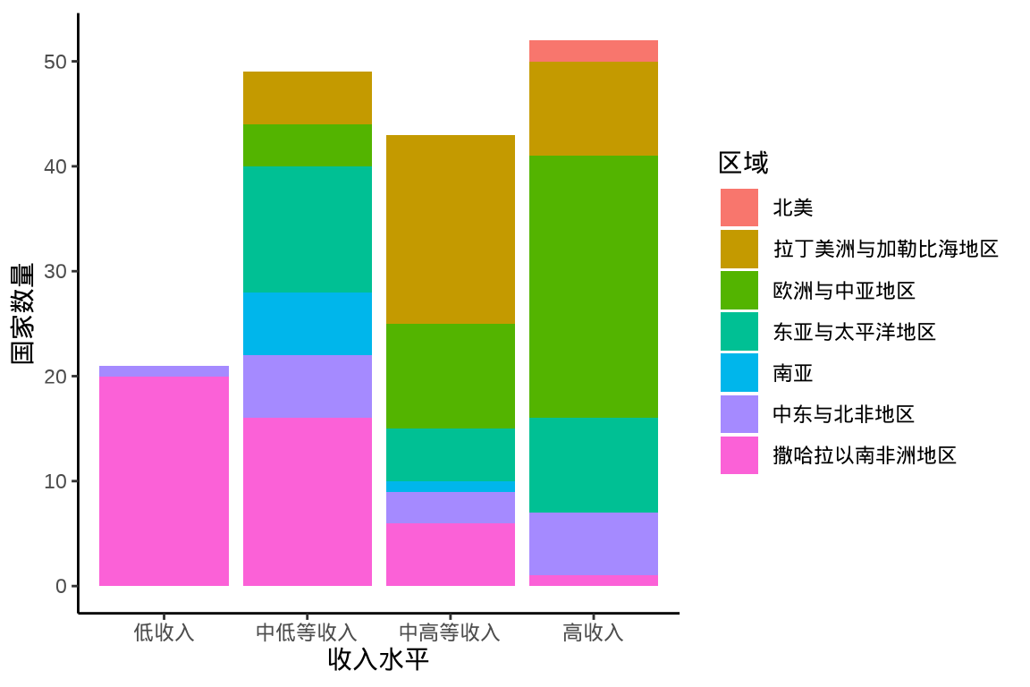
图 1.6: 笛卡尔坐标系下的分组堆积柱形图
笛卡尔坐标系下的分组百分比堆积条形图
ggplot(gapminder_2007, aes(x = income_level, fill = region)) +
  geom_bar(stat = "count", position = "fill") +
  scale_y_continuous(labels = scales::percent) +
  theme_classic() +
  labs(x = "收入水平", y = "国家数量的占比", fill = "区域")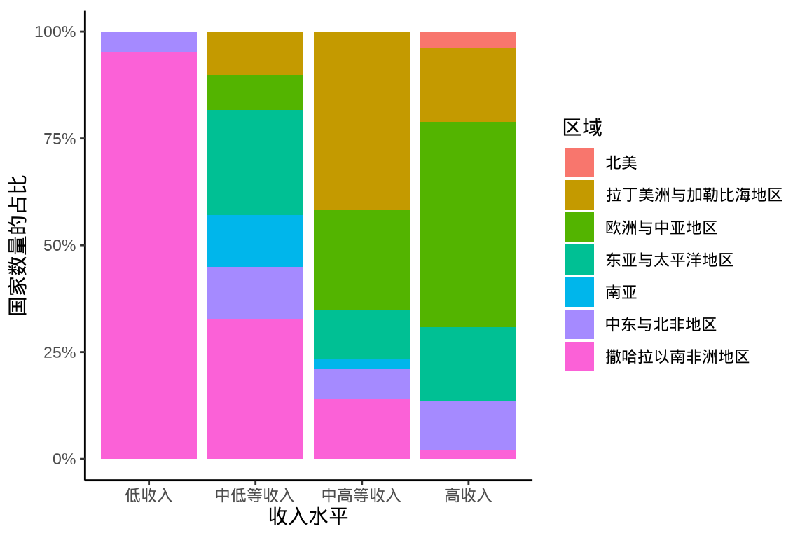
图 1.7: 笛卡尔坐标系下的分组百分比堆积条形图
极坐标系下的分组柱形图
ggplot(gapminder_2007, aes(x = income_level, fill = region)) +
  geom_bar(stat = "count") +
  coord_polar() +
  theme_minimal() +
  labs(x = "收入水平", y = "国家数量", fill = "区域")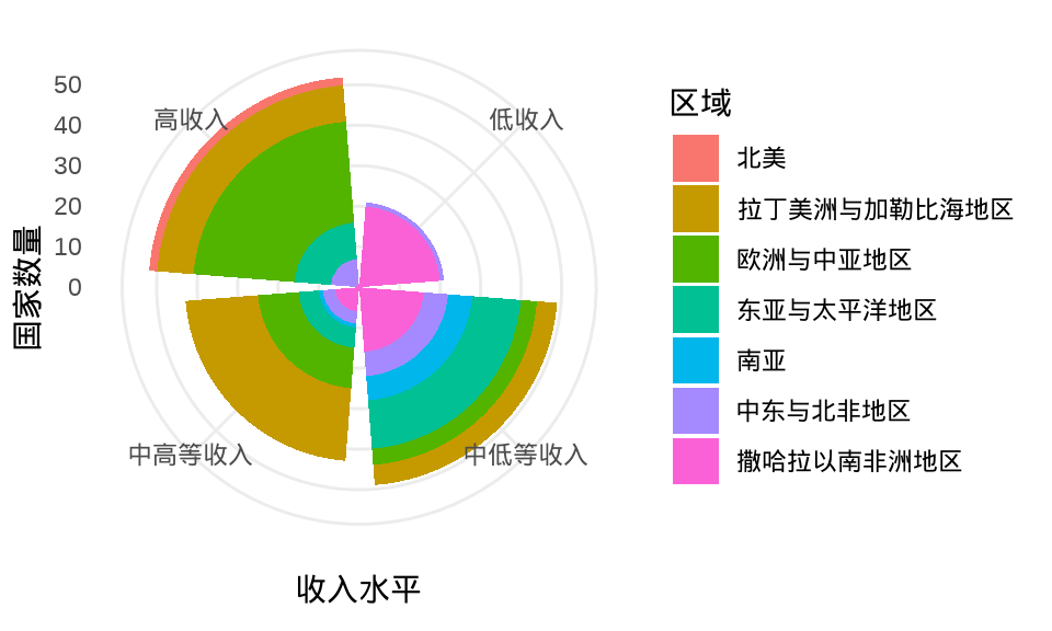
图 1.8: 极坐标系下的分组柱形图
极坐标系下的分组柱形图
ggplot(gapminder_2007, aes(x = income_level, fill = region)) +
  geom_bar(stat = "count", position = "fill") +
  scale_y_continuous(labels = scales::percent) +
  coord_polar() +
  theme_minimal() +
  labs(x = "收入水平", y = "国家数量的占比", fill = "区域")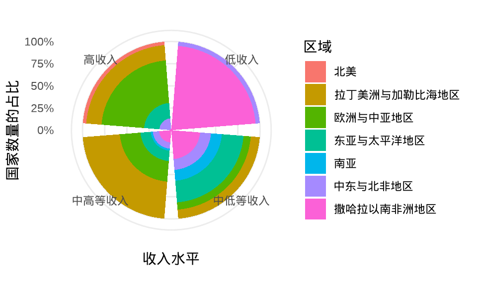
图 1.9: 极坐标系下的分组百分比堆积柱形图
极坐标系下的分组柱形图
ggplot(gapminder_2007, aes(x = income_level, fill = region)) +
  geom_bar(stat = "count") +
  coord_polar(theta = "y") +
  theme_minimal() +
  labs(x = NULL, y = NULL, fill = "区域")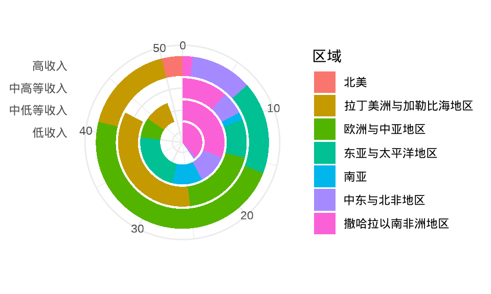
图 1.10: 极坐标系下的分组柱形图
2 插入公式
ggplot2 包内置了一些的数学公式解析和表达能力。形状参数分别为 \(a\) 和 \(b\) 的贝塔分布的概率密度函数如下:
\[ f(x;a,b) = \frac{\Gamma(a+b)}{\Gamma(a)\Gamma(b)}x^{a-1}(1-x)^{b-1}, \quad a>0,b>0,0\leq x \leq 1 \]
2.1 plotmath
Base R 内置的 plotmath 提供一套处理数学公式的方法,详见 ?plotmath。
图2.1 中红线对应贝塔分布 \(B(3,0.9)\) 而蓝线对应贝塔分布 \(B(3,9)\)
ggplot() +
  geom_function(
    fun = dbeta, args = list(shape1 = 3, shape2 = 0.9),
    colour = "#E41A1C", linewidth = 1.2,
  ) +
  geom_function(
    fun = dbeta, args = list(shape1 = 3, shape2 = 9),
    colour = "#377EB8", linewidth = 1.2
  ) +
  theme_classic() +
  labs(
    x = expression(x), y = expression(f(x)),
    title = expression(f(x) == frac(
      Gamma(a + b),
      Gamma(a) * Gamma(b)
    ) * x^{
      a - 1
    } * (1 - x)^{
      b - 1
    })
  )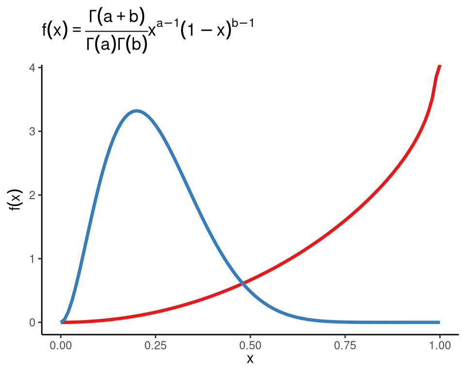
图 2.1: 贝塔分布的概率密度函数
启用 showtext 包会导致数学公式中的括号 () 倾斜,公式和中文混合的情况还不好处理,还不能使用 cairo_pdf 设备保存图形。
2.2 latex2exp
latex2exp 包仍然基于 plotmath,但提供 LaTeX 数学公式的书写方式,相比于 plotmath,使用上会更加方便。
library(latex2exp)
ggplot() +
  geom_function(
    fun = dbeta, args = list(shape1 = 3, shape2 = 0.9),
    colour = "#E41A1C", linewidth = 1.2,
  ) +
  geom_function(
    fun = dbeta, args = list(shape1 = 3, shape2 = 9),
    colour = "#377EB8", linewidth = 1.2
  ) +
  theme_classic() +
  labs(
    x = TeX(r'($x$)'), y = TeX(r'($f(x)$)'),
    title = TeX(r'($f(x) = \frac{\Gamma(a+b)}{\Gamma(a)\Gamma(b)}x^{a-1}(1-x)^{b-1}$)')
  )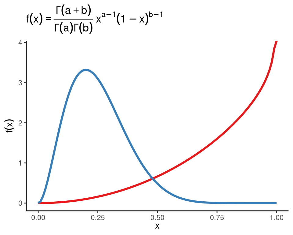
图 2.2: 贝塔分布的概率密度函数
2.3 tikzDevice
Ralf Stubner 维护的 tikzDevice 包提供了另一种嵌入数学字体的方式,其提供的 tikzDevice::tikz() 绘图设备将图形对象转化为 TikZ 代码,调用 LaTeX 引擎编译成 PDF 文档。tikzDevice包大大扩展了数学公式的处理能力,相比于 latex2exp 包,tikzDevice 调用 LaTeX 编译引擎处理数学公式,渲染的公式效果更加精美,支持的数学公式符号更多,不再局限于 plotmath 的能力。
首先安装一些所需的 LaTeX 宏包。
tinytex::tlmgr_install("ctex", "fandol", "standalone", "sourcesanspro", "jknapltx")设置默认的 LaTeX 编译引擎为 XeLaTeX,相比于 PDFLaTeX,它对中文的兼容性更好,支持多平台下的中文环境,中文字体这里采用了开源的 Fandol 字体,默认加载了 mathrsfs 宏包支持 \mathcal、\mathscr 等命令,此外, LaTeX 发行版采用谢益辉自定义的 TinyTeX。推荐的全局 LaTeX 环境配置如下:
options(
  tinytex.engine = "xelatex",
  tikzDefaultEngine = "xetex",
  tikzDocumentDeclaration = "\\documentclass[tikz]{standalone}\n",
  tikzXelatexPackages = c(
    "\\usepackage[fontset=fandol]{ctex}",
    "\\usepackage[default,semibold]{sourcesanspro}",
    "\\usepackage{amsfonts,mathrsfs,amssymb}\n"
  )
)
再测试一下 LaTeX 编译环境是否正常。
tikzDevice::tikzTest()#>
#> Active compiler:
#> /usr/bin/xelatex
#> XeTeX 3.141592653-2.6-0.999993 (TeX Live 2021)
#> kpathsea version 6.3.3#> Measuring dimensions of: A#> Running command: '/usr/bin/xelatex' -interaction=batchmode -halt-on-error -output-directory '/tmp/Rtmp3rzvw0/tikzDevicea892c1f4404' 'tikzStringWidthCalc.tex'#> [1] 7.903确认没有问题后,下面图 2.3 的坐标轴标签,标题,图例等位置都支持数学公式,也支持中文,使用 tikzDevice 打造出版级的效果图。更多功能的介绍见 https://www.daqana.org/tikzDevice/。
library(ggplot2)
ggplot() +
  geom_function(
    fun = dbeta, args = list(shape1 = 3, shape2 = 0.9),
    colour = "#E41A1C", linewidth = 1.5,
  ) +
  geom_function(
    fun = dbeta, args = list(shape1 = 3, shape2 = 9),
    colour = "#377EB8", linewidth = 1.5
  ) +
  theme_classic() +
  labs(
    x = "$x$", y = "$f(x)$",
    title = "$f(x) = \\frac{\\Gamma(a+b)}{\\Gamma(a)\\Gamma(b)}x^{a-1}(1-x)^{b-1}$"
  )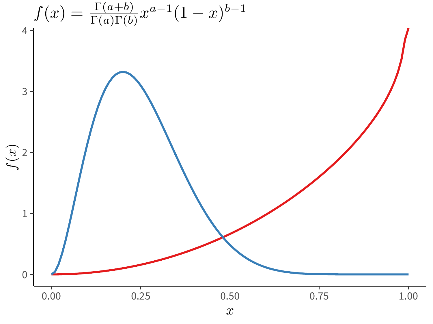
图 2.3: TikZ 渲染的贝塔函数公式
绘制独立的 PDF 图形的过程如下:
library(tikzDevice)
tf <- file.path(getwd(), "tikz-beta.tex")
tikz(tf, width = 3, height = 2.5, pointsize = 30, standAlone = TRUE)
## 绘图代码 ##
dev.off()
# 编译成 PDF 图形
tinytex::latexmk(file = "tikz-beta.tex")
3 设置字体
3.1 Noto 字体
showtext 是一个专用于处理中英文字体的 R 包,支持 Base R 和 ggplot2 绘图,支持调用系统已安装的字体,也支持调用给定路径下的字体,还支持各种奇形怪状的表情字体,更多内容见 (https://github.com/yixuan/showtext),好玩的字体配合好玩的图形,可以玩出很多花样。
## 简体中文宋体字
sysfonts::font_add(
  family = "Noto Serif CJK SC",
  regular = "NotoSerifCJKsc-Regular.otf",
  bold = "NotoSerifCJKsc-Bold.otf"
)
## 无衬线英文字体
sysfonts::font_add(
  family = "Noto Sans",
  regular = "NotoSans-Regular.ttf",
  bold = "NotoSans-Bold.ttf",
  italic = "NotoSans-Italic.ttf",
  bolditalic = "NotoSans-BoldItalic.ttf"
)
接下来查看在当前运行环境下,可供 showtext 包使用的字体。如果配置成功,输出的字体列表中会包含 Noto Serif CJK SC 和 Noto Sans 两款字体。
sysfonts::font_families()#> [1] "sans" "serif" "mono"
#> [4] "Noto Serif CJK SC" "Noto Sans CJK SC" "Noto Serif"
#> [7] "Noto Sans" "wqy-microhei"确认字体配置好了以后,全局默认字体为 Noto 无衬线英文字体,将所有标题处的字体设置为 Noto 系列的简体中文字体。
ggplot(data = gapminder, aes(x = gdpPercap, y = lifeExp)) +
  geom_point(data = function(x) subset(x, year == 2007),
             aes(fill = region, size = pop),
    show.legend = c(fill = TRUE, size = FALSE),
    shape = 21, col = "white"
  ) +
  scale_fill_manual(values = c(
    `拉丁美洲与加勒比海地区` = "#E41A1C", `撒哈拉以南非洲地区` = "#377EB8",
    `欧洲与中亚地区` = "#4DAF4A", `中东与北非地区` = "#984EA3",
    `东亚与太平洋地区` = "#FF7F00", `南亚` = "#FFFF33", `北美` = "#A65628"
  )) +
  scale_size(range = c(2, 12)) +
  scale_x_log10(labels = label_log(), limits = c(100, 110000)) +
  facet_wrap(facets = ~income_level, ncol = 3) +
  theme_classic(base_family = "Noto Sans") +
  theme(
    title = element_text(family = "Noto Serif CJK SC"),
    text = element_text(family = "Noto Serif CJK SC"),
    legend.position =  c(0.9, 0.20)
  ) +
  labs(x = "人均 GDP", y = "预期寿命", fill = "区域")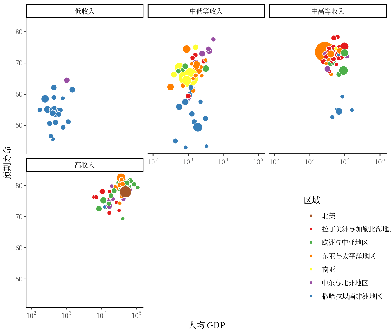
图 3.1: Noto 系列中英文字体
ragg 包 (https://github.com/r-lib/ragg) 无需手动配置字体,只要是系统已经安装的字体,在 ggplot2 绘图时,将字体名称传递给 family 即可。
3.2 Emoji 字体
dat <- data.frame(
  fruits = c("pineapple", "apple", "watermelon", "pear"),
  weight = c(5, 4, 3, 2)
)
# emo 字体
dat$fruits_emo <- sapply(dat$fruits, emo::ji)
ggplot(dat, aes(x = fruits_emo, y = weight)) +
  geom_text(aes(label = fruits_emo),
    size = 12, vjust = -0.5
  ) +
  scale_y_continuous(limits = c(2, 7)) +
  theme_classic() +
  theme(axis.title = element_text(family = "Noto Serif CJK SC")) +
  labs(x = "水果", y = "重量")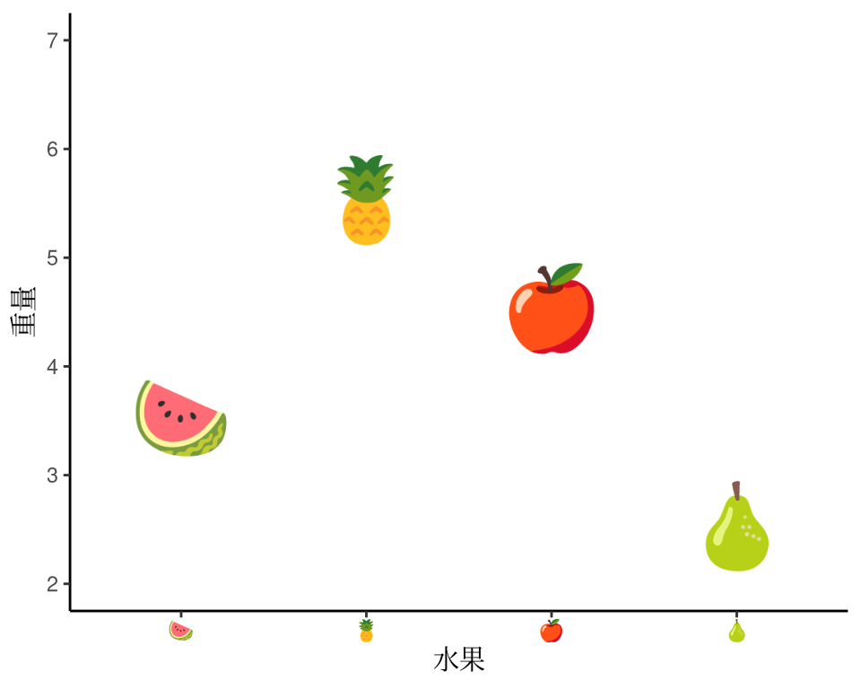
图 3.2: emoji 字体
emojifont 包将 Emoji 字体引入 ggplot2 绘图,如图 3.3 所示。
# emojifont::load.emojifont()
library(emojifont)
dat$fruits_emo <- emojifont::emoji(dat$fruits)
ggplot(dat, aes(x = fruits_emo, y = weight)) +
  geom_text(aes(label = fruits_emo, color = fruits_emo),
    size = 12, vjust = -0.5, family = "EmojiOne", show.legend = FALSE
  ) +
  scale_y_continuous(limits = c(2, 7)) +
  theme_classic() +
  theme(axis.text.x = element_text(size = 20, family = "EmojiOne"),
        axis.text.y = element_text(family = "Noto Sans"),
        axis.title = element_text(family = "Noto Serif CJK SC")) +
  labs(x = "水果", y = "重量")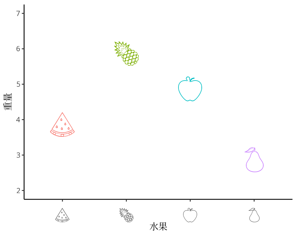
图 3.3: 制作含 Emoji 的图形
先加载 emojifont 包会导致 emo 包无法使用彩色字体,因为 emojifont 自动加载了字体和设备,emo 不能与 showtext 包同时使用。而且 plotmath 数学符号会变形,所以插入公式放在设置字体前面。
加载 emojifont 包会自动加载 Emoji 字体,而从命名空间导入字体
emojifont::load.emojifont()同样会导致插入公式一节不能正常使用
4 制作动画
从 1991 年至2020 年,gapminder 数据集一共是 30 年的数据。 3 根据 2007 年的数据绘制了 3.1 ,每年的数据绘制一幅图像,30 年总共可获得 30 帧图像,再以每秒播放 5 帧图像的速度将 30 帧图像合成 GIF 动画。因此,设置这个动画总共 30 帧,每秒播放的图像数为 5。
options(gganimate.nframes = 30, gganimate.fps = 5)gganimate 包提供一套代码风格类似 ggplot2 包的动态图形语法,可以非常顺滑地与之连接。在了解了 ggplot2 绘制图形的过程后,用 gganimate 包制作动画是非常容易的。gganimate 包会调用 gifski (https://github.com/r-rust/gifski) 包来合成动画,因此,除了安装 gganimate 包,还需要安装 gifski 包。接着,在已有的 ggplot2 绘图代码基础上,再追加一个转场图层函数 transition_time(),这里是按年逐帧展示图像,因此,其转场的时间变量为 gapminder 数据集中的变量 year。
library(gganimate)
ggplot(data = gapminder, aes(x = gdpPercap, y = lifeExp)) +
  geom_point(aes(color = region, size = pop),
    show.legend = c(color = TRUE, size = TRUE)
  ) +
  scale_color_manual(values = c(
    `拉丁美洲与加勒比海地区` = "#E41A1C", `撒哈拉以南非洲地区` = "#377EB8",
    `欧洲与中亚地区` = "#4DAF4A", `中东与北非地区` = "#984EA3",
    `东亚与太平洋地区` = "#FF7F00", `南亚` = "#FFFF33", `北美` = "#A65628"
  )) +
  scale_size(range = c(2, 12), labels = label_number(scale_cut = cut_short_scale())) +
  scale_x_log10(labels = label_log(), limits = c(10, 130000)) +
  facet_wrap(facets = ~income_level) +
  theme_classic(base_family = "Noto Sans") +
  theme(
    title = element_text(family = "Noto Serif CJK SC"),
    text = element_text(family = "Noto Serif CJK SC")
  ) +
  labs(
    title = "{frame_time} 年", x = "人均 GDP",
    y = "预期寿命", size = "人口总数", color = "区域"
  ) +
  transition_time(time = year)
ggplot(data = gapminder, aes(x = gdpPercap, y = lifeExp)) +
  geom_point(aes(color = income_level, size = pop),
    show.legend = c(color = TRUE, size = TRUE)
  ) +
  scale_color_brewer(palette = "RdYlGn") +
  scale_radius(range = c(1, 6), trans = "log10",
             labels = label_number(scale_cut = cut_short_scale())) +
  scale_x_log10(labels = label_log(), limits = c(10, 130000)) +
  facet_wrap(facets = ~region, ncol = 3) +
  theme_classic(base_family = "Noto Sans") +
  theme(
    title = element_text(family = "Noto Serif CJK SC"),
    text = element_text(family = "Noto Serif CJK SC")
  ) +
  labs(
    title = "{frame_time} 年", x = "人均 GDP",
    y = "预期寿命", size = "人口总数", color = "收入水平"
  ) +
  transition_time(time = year)
去掉分面
# 刻度线位置
mb <- unique(as.numeric(1:10 %o% 10^(1:4)))
ggplot(data = gapminder, aes(x = gdpPercap, y = lifeExp)) +
  geom_point(aes(color = region, size = pop),
             show.legend = c(color = TRUE, size = TRUE)
  ) +
  scale_color_manual(values = c(
    `拉丁美洲与加勒比海地区` = "#E41A1C", `撒哈拉以南非洲地区` = "#377EB8",
    `欧洲与中亚地区` = "#4DAF4A", `中东与北非地区` = "#984EA3",
    `东亚与太平洋地区` = "#FF7F00", `南亚` = "#FFFF33", `北美` = "#A65628"
  )) +
  scale_radius(range = c(1, 6), trans = "log10",
             labels = label_number(scale_cut = cut_short_scale())) +
  scale_x_log10(labels = label_dollar(), minor_breaks = mb, limits = c(10, 130000)) +
  scale_y_continuous(n.breaks = 6) +
  theme_classic(base_family = "Noto Sans") +
  theme(
    title = element_text(family = "Noto Serif CJK SC"),
    text = element_text(family = "Noto Serif CJK SC"),
    panel.grid.major = element_line(),
    panel.grid.minor.x = element_line()
  ) +
  labs(
    title = "{frame_time} 年", x = "人均 GDP",
    y = "预期寿命", size = "人口总数", color = "区域"
  ) +
  transition_time(time = year)
5 组合图形
patchwork 包提供了一套非常简洁的语法,用来组合多个 ggplot2 图形。如图 5.1 所示,用散点图分别绘制 2002 年和 2007 年的数据,并将图形肩并肩的并排展示。
p1 <- ggplot(data = gapminder, aes(x = gdpPercap, y = lifeExp)) +
  geom_point(data = function(x) subset(x, year == 2020),
             aes(color = income_level, size = pop)) +
  scale_color_brewer(palette = "RdYlGn") +
  scale_radius(range = c(1, 6), trans = "log10",
               labels = label_number(scale_cut = cut_short_scale())) +
  scale_x_log10(labels = label_log(), limits = c(10, 130000)) +
  theme_minimal() +
  labs(
    title = "2020 年", x = "人均 GDP",
    y = "预期寿命", size = "人口总数", color = "收入水平"
  )

p2 <- ggplot(data = gapminder, aes(x = gdpPercap, y = lifeExp)) +
  geom_point(data = function(x) subset(x, year == 2010),
             aes(color = income_level, size = pop)) +
  scale_color_brewer(palette = "RdYlGn") +
  scale_radius(range = c(1, 6), trans = "log10",
               labels = label_number(scale_cut = cut_short_scale())) +
  scale_x_log10(labels = label_log(), limits = c(10, 130000)) +
  theme_minimal() +
  labs(
    title = "2010 年", x = "人均 GDP",
    y = "预期寿命", size = "人口总数", color = "收入水平"
  )

library(patchwork)
p1 | p2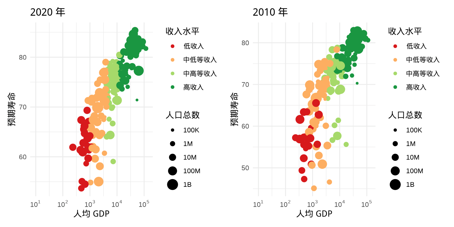
图 5.1: 左右组合
除了用竖线 | 左右并排,还可以用斜杠 / 做上下排列,见下图 5.2 。
p1 / p2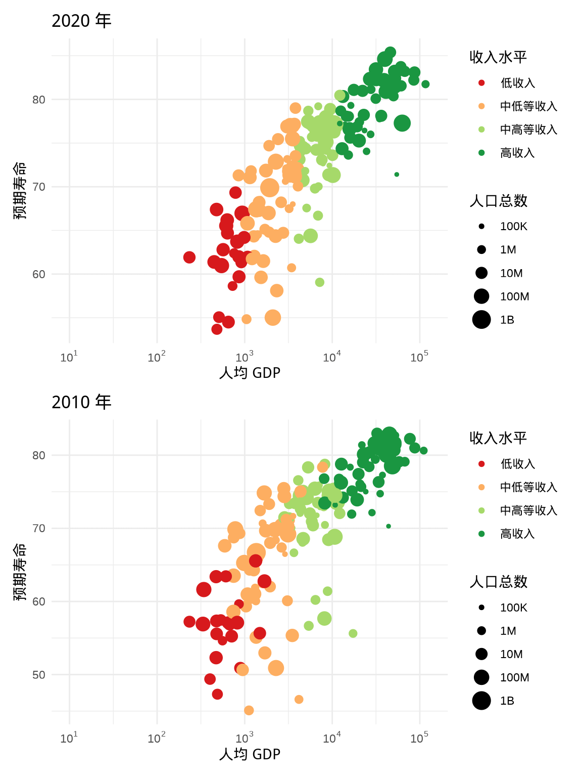
图 5.2: 上下组合
还可以引入括号 (),实现更加复杂的图形组合,见下图 5.3 。
p3 <- ggplot(data = gapminder, aes(x = gdpPercap, y = lifeExp)) +
  geom_point(data = function(x) subset(x, year == 2000),
             aes(color = income_level, size = pop)) +
  scale_color_brewer(palette = "RdYlGn") +
  scale_radius(range = c(1, 6), trans = "log10",
               labels = label_number(scale_cut = cut_short_scale())) +
  scale_x_log10(labels = label_log(), limits = c(10, 130000)) +
  theme_minimal() +
  labs(
    title = "2000 年", x = "人均 GDP",
    y = "预期寿命", size = "人口总数", color = "收入水平"
  )

p1 / (p2 | p3)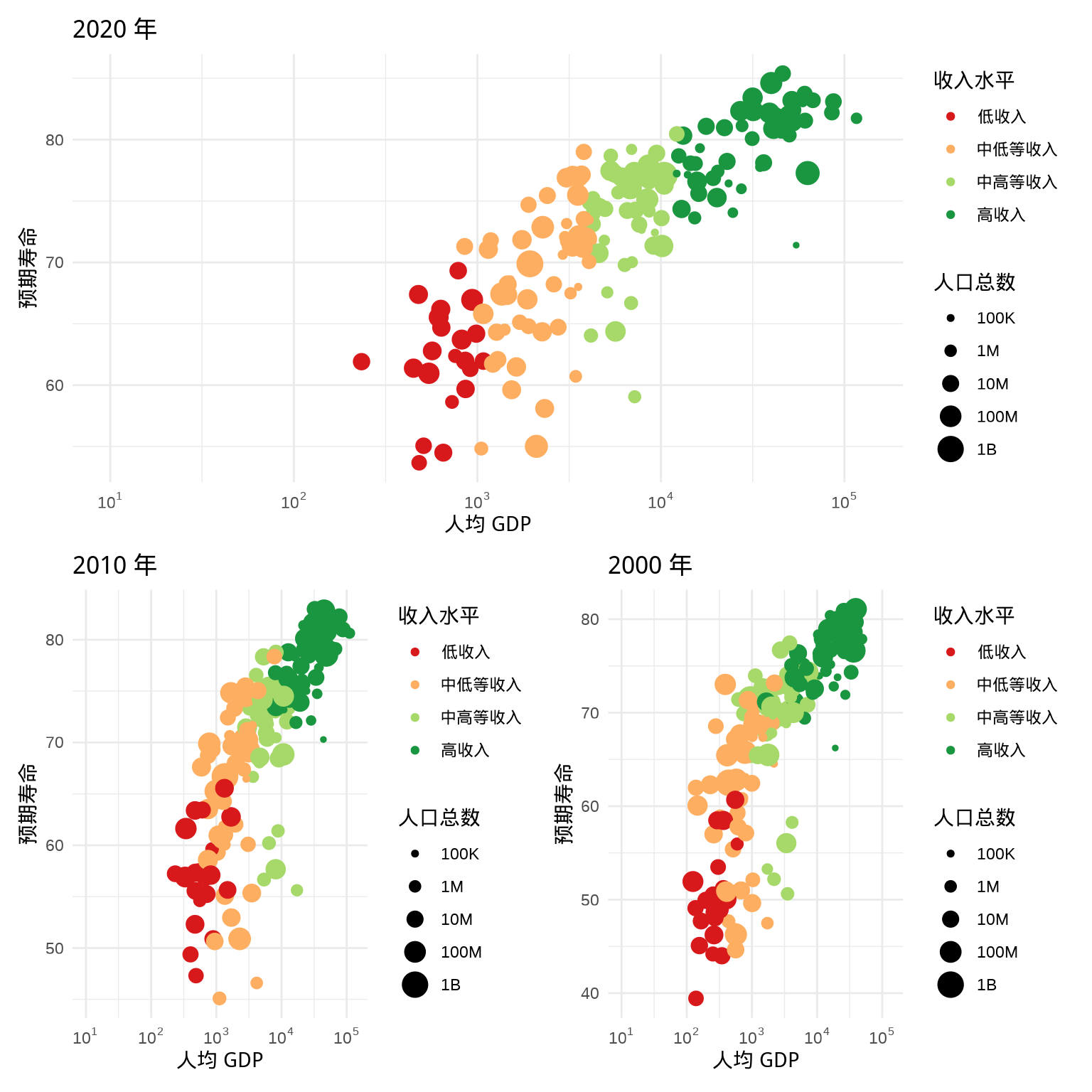
图 5.3: 多图组合
结合上面的介绍,不难看出,竖线 | 用于左右分割,斜杠 / 用于上下分割,而括号 () 用于范围的限定,下图 5.4 是去掉括号后的效果。
p1 / p2 | p3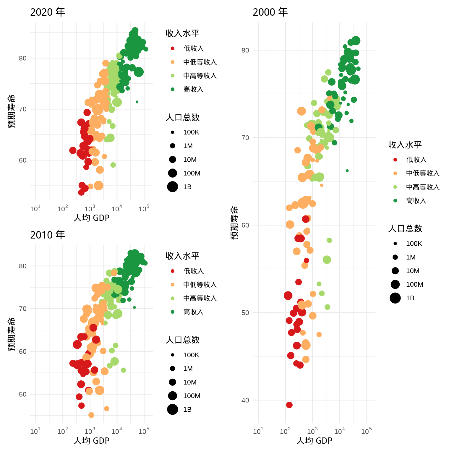
图 5.4: 多图组合
还可以将图例收集起来,合并放置在一处。p1 、p2 和 p3 的图例是一样的,可以将 p2 和 p3 的图例隐藏起来,将 p1 的图例放置在右侧居中的位置。
p4 <- p2 +
  theme(legend.position = "none")
p5 <- p3 +
  theme(legend.position = "none")
p1 / (p4 | p5) +
  plot_layout(guides = "collect")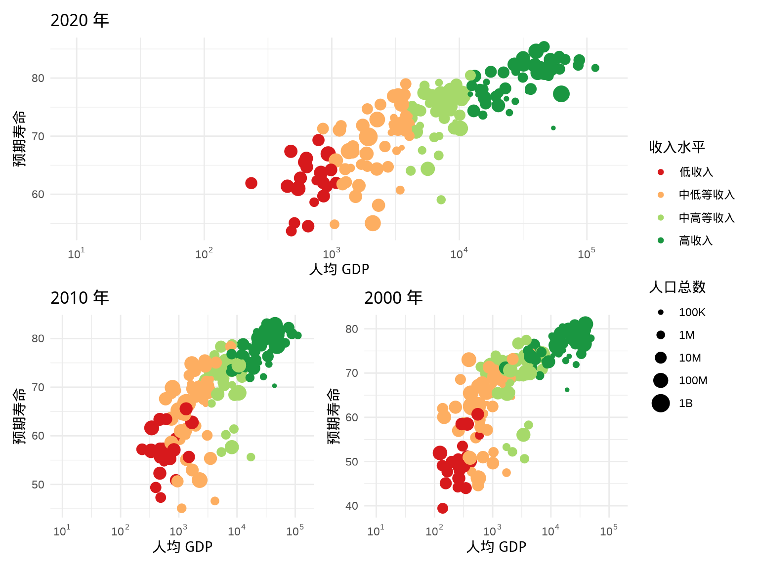
图 5.5: 多图组合
看起来,有点像分面绘图,但是一个图占两列又表示它不是分面绘图,而是多图布局的效果。
最常用的功能就是这些啦,更多内容可以去 patchwork 包官网了解。其它可以用来组合多个 ggplot2 图形的 R 包有 cowplot (https://github.com/wilkelab/cowplot)、gridExra (https://cran.r-project.org/package=gridExtra) 和 gghalves (https://github.com/erocoar/gghalves) 等。
6 保存图形
ggplot2 包提供保存图形的函数 ggsave(),它可以将 ggplot2 对象导出为各种格式的图片,比如 PNG 位图图片、 SVG 矢量图片等。
p <- ggplot(gapminder_2007, aes(x = gdpPercap, y = lifeExp)) +
  geom_point(aes(color = income_level)) +
  scale_x_log10(labels = scales::label_log()) +
  theme_classic()
位图是由像素(Pixel)构成的,单位 units 是 px,分辨率取决于单位面积上像素的数量,参数 dpi 往往根据显示设备而定,出版打印常用 300。
ggsave(filename = "gapminder.png", plot = p,
       width = 800, height = 600, units = "px",
       device = "png", dpi = 300)
矢量图是由点构成的,由点及线,由线构成路径,在一定坐标系统下,每个点都记录了坐标及方向。
ggsave(filename = "gapminder.svg", plot = p,
       width = 8, height = 6, units = "in",
       device = "svg")
7 图文混合
geomtextpath 包新添文本路径图层,文本随路径变化,实现图文混合的效果,也省了图例,如图 7.1 所示。
library(geomtextpath)
ggplot(gapminder_2007, aes(x = gdpPercap, y = lifeExp,
                           color = income_level)) +
  geom_point(show.legend = FALSE) +
  scale_x_log10(labels = scales::label_log()) +
  geom_labelsmooth(aes(label = year),
    text_smoothing = 30, fill = "#F6F6FF",
    method = "lm", formula = y ~ log10(x), show.legend = FALSE,
    size = 4, linewidth = 1, boxlinewidth = 0.3
  ) +
  theme_classic() +
  labs(
    title = "2007 年", x = "人均 GDP",
    y = "预期寿命", color = "收入水平"
  )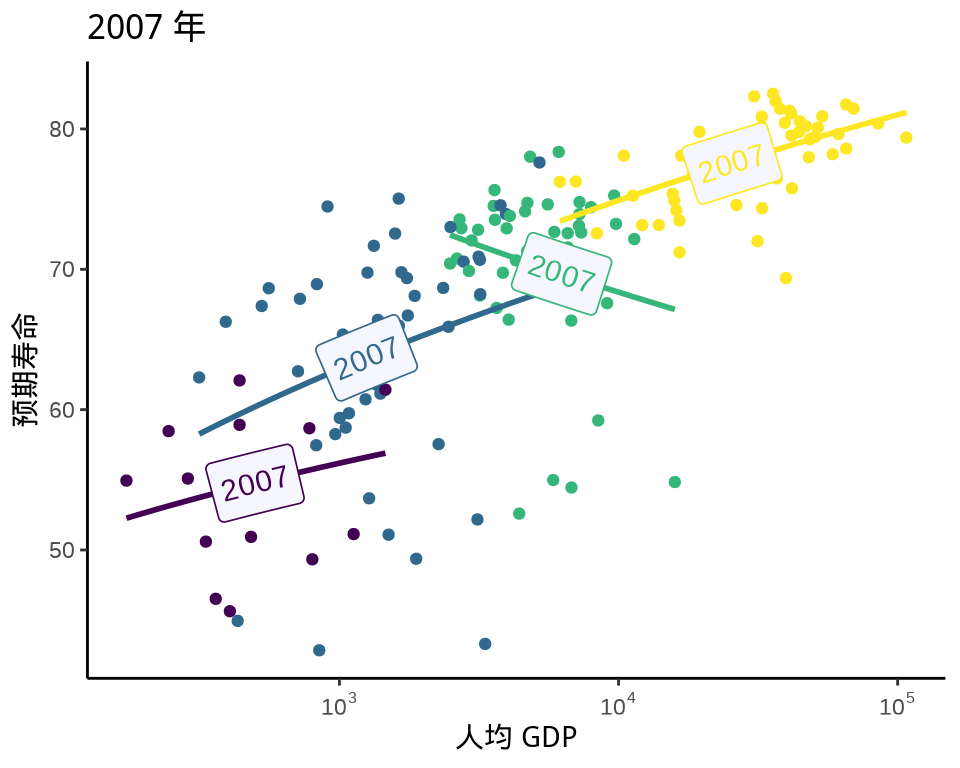
图 7.1: 图文混合
8 局部缩放
局部缩放是非常常用的一个绘图需求,有时候就是需要将局部细节放大,再绘制,以展示图形的重点关注区域。 ggforce 包的 facet_zoom() 函数将目标区域作为单独的一个分面展示。
library(ggforce)
ggplot(gapminder_2007, aes(x = gdpPercap, y = lifeExp)) +
  geom_point(aes(colour = income_level)) +
  facet_zoom(x = income_level == "低收入") +
  labs(x = "人均 GDP", y = "预期寿命", color = "收入水平")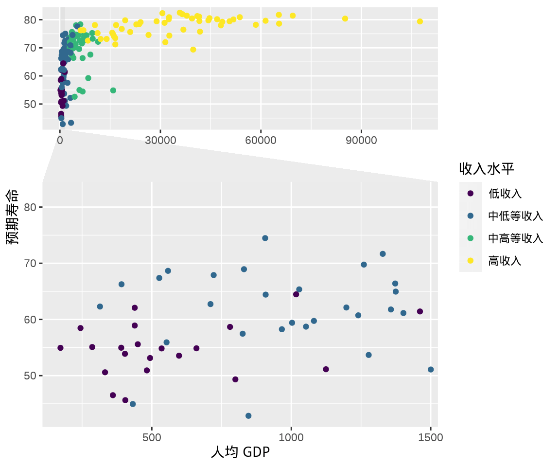
图 8.1: 局部缩放
9 添加水印
patchwork 包的函数 inset_element() 可以给图片上添加某公司的徽标或水印文字,以示版权归属。
# 绘图展示数据
p <- ggplot(gapminder_2007, aes(x = gdpPercap, y = lifeExp)) +
  geom_point(aes(color = income_level)) +
  scale_x_log10(labels = scales::label_log()) +
  theme_classic() +
  labs(x = "人均 GDP", y = "预期寿命", color = "收入水平")
# 提供水印图片
logo_file <- system.file("help", "figures", "logo.png",
                         package = "patchwork")
# 读取 PNG 图片
img <- png::readPNG(logo_file, native = TRUE)
# 添加水印图片
p + inset_element(
  p = img,
  left = 0.8,
  bottom = 0.8,
  right = 1,
  top = 1,
  align_to = "full"
)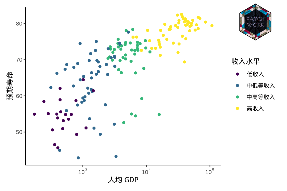
图 9.1: 添加水印图片和文字
10 表情符号
ggChernoff 包受 Chernoff 表达多元数据的启发,借助从笑脸到苦脸的 Emoji 表情符号来表达数据指标。比如从低收入到高收入的连续型数据,从非常喜欢到非常不喜欢的有序分类型数据,用表情表达此类数据,显得非常形象。下图 10.1 以收入水平分类,在每个分类中,将预期寿命与表情结合,越长寿越开心。
library(ggChernoff)
library(data.table)
gapminder_2007 <- as.data.table(gapminder_2007)
gapminder_2007[, smile := scales::rescale(lifeExp), by = "income_level"]

ggplot(gapminder_2007, aes(x = gdpPercap, y = lifeExp)) +
  geom_chernoff(aes(smile = smile, fill = income_level),
                alpha = 0.85, color = "white",
                show.legend = c(smile = FALSE, fill = TRUE)) +
  scale_x_log10(labels = scales::label_log()) +
  scale_fill_brewer(palette = "Spectral",
                    guide = guide_legend(reverse = TRUE)) +
  scale_smile_continuous(midpoint = 0.5) +
  theme_classic() +
  labs(x = "人均 GDP", y = "预期寿命", fill = "收入水平")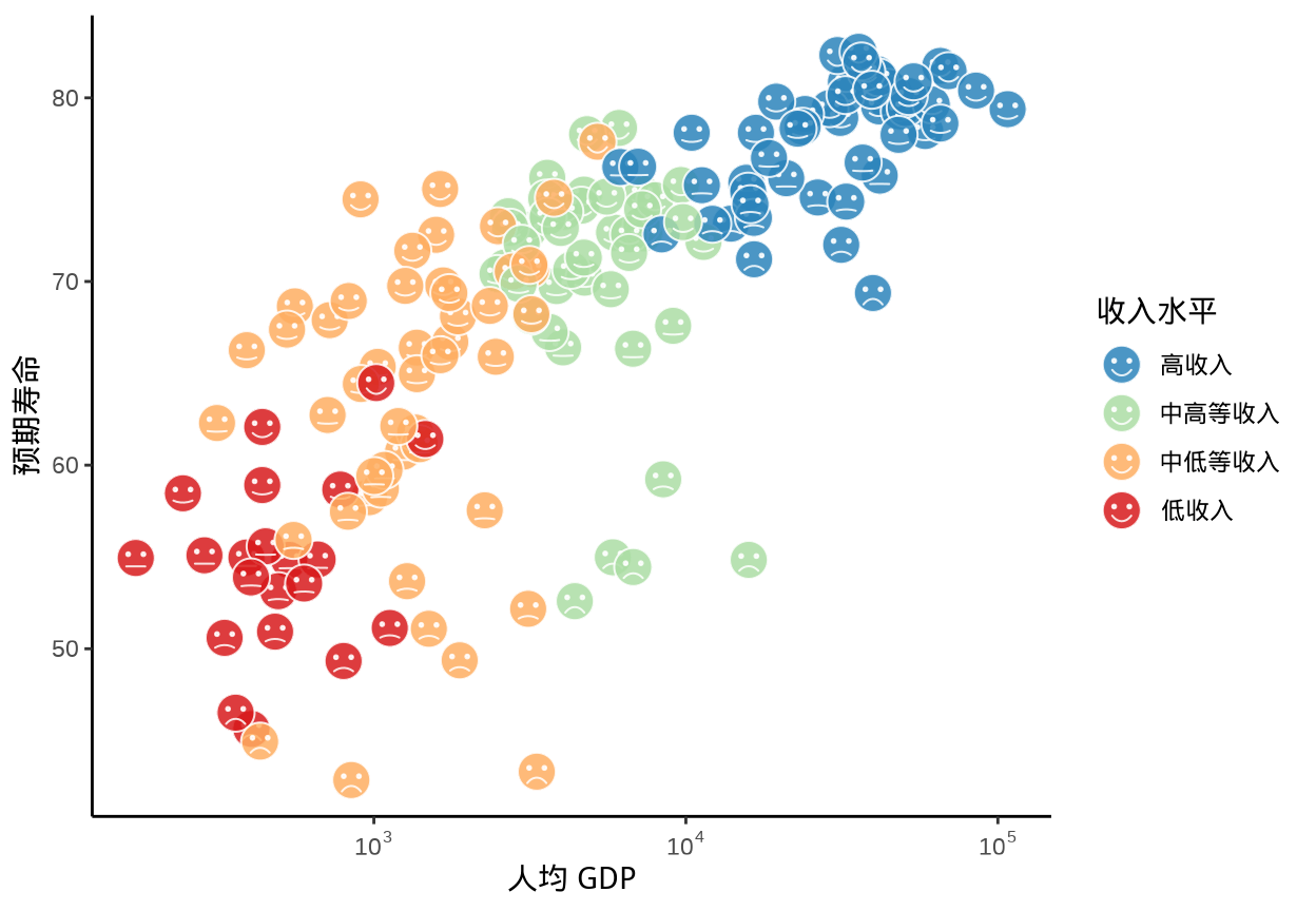
图 10.1: 切尔诺夫脸谱图
11 环境信息
在 RStudio IDE 内编辑本文的 R Markdown 源文件,用 blogdown 构建网站,Hugo 渲染 knitr 之后的 Markdown 文件,得益于 blogdown 对 R Markdown 格式的支持,图、表和参考文献的交叉引用非常方便,省了不少文字编辑功夫。文中使用了多个 R 包,为方便复现本文内容,下面列出详细的环境信息:
xfun::session_info()#> R version 4.2.2 (2022-10-31)
#> Platform: x86_64-redhat-linux-gnu (64-bit)
#> Running under: Fedora Linux 37 (Container Image)
#>
#> Locale:
#> LC_CTYPE=en_US.UTF-8 LC_NUMERIC=C
#> LC_TIME=en_US.UTF-8 LC_COLLATE=en_US.UTF-8
#> LC_MONETARY=en_US.UTF-8 LC_MESSAGES=en_US.UTF-8
#> LC_PAPER=en_US.UTF-8 LC_NAME=C
#> LC_ADDRESS=C LC_TELEPHONE=C
#> LC_MEASUREMENT=en_US.UTF-8 LC_IDENTIFICATION=C
#>
#> Package version:
#> askpass_1.1 assertthat_0.2.1 base64enc_0.1.3
#> blogdown_1.16 bookdown_0.32 bslib_0.4.2
#> cachem_1.0.6 cli_3.6.0 colorspace_2.1-0
#> compiler_4.2.2 cpp11_0.4.3 crayon_1.5.2
#> curl_5.0.0 data.table_1.14.8 digest_0.6.31
#> dplyr_1.1.0 ellipsis_0.3.2 emo_0.0.0.9000
#> emojifont_0.5.5 evaluate_0.20 fansi_1.0.4
#> farver_2.1.1 fastmap_1.1.0 filehash_2.4-5
#> fs_1.6.1 generics_0.1.3 geomtextpath_0.1.1
#> gganimate_1.0.8 ggChernoff_0.3.0 ggforce_0.4.1
#> ggplot2_3.4.1 gifski_1.6.6-1 glue_1.6.2
#> graphics_4.2.2 grDevices_4.2.2 grid_4.2.2
#> gtable_0.3.1 highr_0.10 hms_1.1.2
#> htmltools_0.5.4 httpuv_1.6.9 isoband_0.2.7
#> jquerylib_0.1.4 jsonlite_1.8.4 knitr_1.42
#> labeling_0.4.2 later_1.3.0 latex2exp_0.9.6
#> lattice_0.20-45 lifecycle_1.0.3 lubridate_1.9.2
#> magick_2.7.3 magrittr_2.0.3 MASS_7.3-58.2
#> Matrix_1.5-3 memoise_2.0.1 methods_4.2.2
#> mgcv_1.8-41 mime_0.12 munsell_0.5.0
#> nlme_3.1-162 patchwork_1.1.2 pdftools_3.3.3
#> pillar_1.8.1 pkgconfig_2.0.3 png_0.1-8
#> polyclip_1.10-4 prettyunits_1.1.1 progress_1.2.2
#> promises_1.2.0.1 proto_1.0.0 purrr_1.0.1
#> qpdf_1.3.0 R6_2.5.1 ragg_1.2.5
#> rappdirs_0.3.3 RColorBrewer_1.1-3 Rcpp_1.0.10
#> RcppEigen_0.3.3.9.3 rlang_1.0.6 rmarkdown_2.20
#> rstudioapi_0.14 sass_0.4.5 scales_1.2.1
#> servr_0.25 showtext_0.9-5 showtextdb_3.0
#> splines_4.2.2 stats_4.2.2 stringi_1.7.12
#> stringr_1.5.0 sys_3.4.1 sysfonts_0.8.8
#> systemfonts_1.0.4 textshaping_0.3.6 tibble_3.1.8
#> tidyselect_1.2.0 tikzDevice_0.12.4 timechange_0.2.0
#> tinytex_0.44 tools_4.2.2 tweenr_2.0.2
#> utf8_1.2.3 utils_4.2.2 vctrs_0.5.2
#> viridisLite_0.4.1 withr_2.5.0 xfun_0.37
#> yaml_2.3.7