1 本文背景

自 1997 年 9 月 18 日 Ross Ihaka 在 Apache Subversion（下面简称 SVN）上提交第一次代码以来，R 语言的开发一直由 R Core Team（即 R 语言核心团队）在 SVN 上进行着，到如今 25 年快过去了。25 年，四分之一个世纪，Brian Ripley 大人一路陪伴 R 语言的成长，如今，70 岁了，还在继续！

本文将分析 Brian Ripley 在 SVN 上留下的一段足迹，观察陪跑的一段历程 — 2003 至 2012 的十年，也正是 R 语言蓬勃发展的十年。R 语言开发者网站(https://developer.r-project.org/)提供了一份逐年的代码提交日志，官网除了提供日志数据直接下载地址，也提供了日志数据的生成过程，简单来说，就是从代码版本管理工具 SVN 中抽出来，下面的代码可以查看最近两天的提交日志。

## 笔者在 MacOS 上请测可用
svn log -v -r HEAD:\{`date +%Y-%m-%d`\} https://svn.r-project.org/R

本文将完全基于 R 语言实现日志数据的分析过程，且保证代码稳定可重复。数据预处理的步骤有：读取文本数据，借助正则表达式匹配、筛选、抽取。仅说明每段代码的作用，而略去单个函数的介绍。分析过程中主要涉及的工具有：Base R 数据操作，lattice [1] 数据可视化，期间穿插笔者的一些分析，希望对读者有所启发。

2 数据准备

目前，R 语言源码及开发一直都在 SVN 上，在 Github 上有一份源码镜像，保持持续同步，R 语言官方网站及博客源码数据存放在 Github (https://github.com/r-devel/r-dev-web)。

2003-2012 年的日志数据是现成的，总计约 10 年的 SVN 提交日志数据，先从 R 语言官网下载，保存到本地文件夹 data-raw/，然后批量导入数据到 R 环境。读者可先查看其中一个文件的数据，直观了解数据的形态，分析探索之旅将从这里出发。

2.1 查看数据

查看纯文本文件 R_svnlog_2003 的头 10 行记录，即 2003 年 CRAN 团队代码提交日志数据。

## 命令行窗口中查看文件前 10 行数据
head -n 10 data-raw/R_svnlog_2003

------------------------------------------------------------------------
r27839 | pd | 2003-12-31 18:35:40 -0500 (Wed, 31 Dec 2003) | 2 lines
Changed paths:
   M /trunk/BUGS

auto-update

------------------------------------------------------------------------
r27838 | pd | 2003-12-31 18:35:35 -0500 (Wed, 31 Dec 2003) | 2 lines
Changed paths:

# 批量导入原始数据到 R 环境
meta_data <- unlist(lapply(
  list.files(
    path = "data-raw",
    full.names = T,
    pattern = "R_svnlog_\\d{4}"
  ), readLines
))

查看导入 R 环境中的数据情况

writeLines(meta_data[1:15])

------------------------------------------------------------------------
r27839 | pd | 2003-12-31 18:35:40 -0500 (Wed, 31 Dec 2003) | 2 lines
Changed paths:
   M /trunk/BUGS

auto-update

------------------------------------------------------------------------
r27838 | pd | 2003-12-31 18:35:35 -0500 (Wed, 31 Dec 2003) | 2 lines
Changed paths:
   M /branches/R-1-8-patches/BUGS

auto-update

------------------------------------------------------------------------

2.2 筛选数据

不难看出，每一条 SVN 提交日志用虚线分割，本文主要关注：

## 提交代码的 ID commit_id、贡献者 contributor、时间戳 timestamp 和修改行数 lines
r27838 | pd | 2003-12-31 18:35:35 -0500 (Wed, 31 Dec 2003) | 2 lines

按照时间戳的格式过滤出提交日志的信息，比如 2003-12-31 18:35:35。

## 过滤出想要的文本
filter_meta_data <- meta_data[grepl(pattern = "(\\d{4}-\\d{2}-\\d{2} \\d{2}:\\d{2}:\\d{2})", x = meta_data)]

它们是用竖线分割的文本数据，只需将字符串按此规律分割，即可提取各个字段。

## 分割文本
split_meta_data <- strsplit(x = filter_meta_data, split = " | ", fixed = T)

接下来整理成适合进行数据操作的数据类型。

## 构造 matrix 类型
tidy_meta_data <- matrix(
  data = unlist(split_meta_data), ncol = 4, byrow = T,
  dimnames = list(c(), c("commit_id", "contributor", "timestamp", "lines"))
)
## 转化为 data.frame
tidy_meta_data <- as.data.frame(tidy_meta_data)

2.3 抽取数据

为了提取文本数据中的有效信息，先准备一个提取函数。

## 从一段文本中，按照给定的匹配模式提取一部分文本 
str_extract <- function(text, pattern, ...) regmatches(text, regexpr(pattern, text, ...))

提取代码提交时间和修改代码行数。

# 提取时间戳和代码修改行数
spread_meta_data <- within(tidy_meta_data, {
  time <- str_extract(text = timestamp, pattern = "\\d{4}-\\d{2}-\\d{2} \\d{2}:\\d{2}:\\d{2}")
  cnt <- str_extract(text = lines, pattern = "\\d{1}")
})

2.4 数据转换

再进行一些必要的数据转化，提取时间信息

# 代码行数转为整型
spread_meta_data$cnt <- as.integer(spread_meta_data$cnt)
# 时间戳用 POSIXlt 类型表示
spread_meta_data$time <- as.POSIXlt(spread_meta_data$time, format = "%Y-%m-%d %H:%M:%S", tz = "UTC")
# 提取日期
spread_meta_data$date <- format(spread_meta_data$time, format = "%Y-%m-%d", tz = "UTC")
# 提取年份
spread_meta_data$year <- format(spread_meta_data$time, format = "%Y", tz = "UTC")
# 提取月份
spread_meta_data$month <- format(spread_meta_data$time, format = "%m", tz = "UTC")
# 提取时段
spread_meta_data$hour <- format(spread_meta_data$time, format = "%H", tz = "UTC")
# 时段转为整型
spread_meta_data$hour <- as.integer(spread_meta_data$hour)
# 一周的周几
spread_meta_data$weekday <- weekdays(spread_meta_data$time, abbreviate = T)
# 转为 factor 类型
spread_meta_data$weekday <- factor(spread_meta_data$weekday,
  levels = c("Mon", "Tue", "Wed", "Thu", "Fri", "Sat", "Sun")
)
# 一年的第几天
spread_meta_data$days <- format(spread_meta_data$time, format = "%j", tz = "UTC")
# 转为整型，一年总共 300 多天，整型够用
spread_meta_data$days <- as.integer(spread_meta_data$days)

查看整理后的数据，如下：

# 数据类型
str(spread_meta_data)

## 'data.frame':    38954 obs. of  12 variables:
##  $ commit_id  : chr  "r27839" "r27838" "r27837" "r27836" ...
##  $ contributor: chr  "pd" "pd" "ripley" "jmc" ...
##  $ timestamp  : chr  "2003-12-31 18:35:40 -0500 (Wed, 31 Dec 2003)" "2003-12-31 18:35:35 -0500 (Wed, 31 Dec 2003)" "2003-12-31 12:58:22 -0500 (Wed, 31 Dec 2003)" "2003-12-31 11:22:43 -0500 (Wed, 31 Dec 2003)" ...
##  $ lines      : chr  "2 lines" "2 lines" "2 lines" "2 lines" ...
##  $ cnt        : int  2 2 2 2 4 2 2 2 2 3 ...
##  $ time       : POSIXlt, format: "2003-12-31 18:35:40" "2003-12-31 18:35:35" ...
##  $ date       : chr  "2003-12-31" "2003-12-31" "2003-12-31" "2003-12-31" ...
##  $ year       : chr  "2003" "2003" "2003" "2003" ...
##  $ month      : chr  "12" "12" "12" "12" ...
##  $ hour       : int  18 18 12 11 11 11 11 6 6 5 ...
##  $ weekday    : Factor w/ 7 levels "Mon","Tue","Wed",..: 3 3 3 3 3 3 3 3 3 3 ...
##  $ days       : int  365 365 365 365 365 365 365 365 365 365 ...

# 前几行数据记录
head(spread_meta_data)

##   commit_id contributor                                    timestamp   lines
## 1    r27839          pd 2003-12-31 18:35:40 -0500 (Wed, 31 Dec 2003) 2 lines
## 2    r27838          pd 2003-12-31 18:35:35 -0500 (Wed, 31 Dec 2003) 2 lines
## 3    r27837      ripley 2003-12-31 12:58:22 -0500 (Wed, 31 Dec 2003) 2 lines
## 4    r27836         jmc 2003-12-31 11:22:43 -0500 (Wed, 31 Dec 2003) 2 lines
## 5    r27835         jmc 2003-12-31 11:22:13 -0500 (Wed, 31 Dec 2003) 4 lines
## 6    r27834         jmc 2003-12-31 11:20:09 -0500 (Wed, 31 Dec 2003) 2 lines
##   cnt                time       date year month hour weekday days
## 1   2 2003-12-31 18:35:40 2003-12-31 2003    12   18     Wed  365
## 2   2 2003-12-31 18:35:35 2003-12-31 2003    12   18     Wed  365
## 3   2 2003-12-31 12:58:22 2003-12-31 2003    12   12     Wed  365
## 4   2 2003-12-31 11:22:43 2003-12-31 2003    12   11     Wed  365
## 5   4 2003-12-31 11:22:13 2003-12-31 2003    12   11     Wed  365
## 6   2 2003-12-31 11:20:09 2003-12-31 2003    12   11     Wed  365

2.5 保存数据

清理完成后，将数据保存起来，以备后用。

## CRAN 团队 SVN 提交日志数据
saveRDS(spread_meta_data, file = "data/cran-svn-log.rds")

3 数据分析

3.1 CRAN 团队

3.1.1 提交量排序（成员）

笔者已迫不及待地想看下这 10 年 R 语言核心团队各个贡献者提交代码的总量，这可以用分组计数实现。

## 按贡献者分组统计提交次数
aggr_meta <- aggregate(x = commit_id ~ contributor, data = spread_meta_data, FUN = function(x) length(unique(x)))

下面简单排个序：

## 按提交次数降序排列
aggr_meta[order(aggr_meta$commit_id, decreasing = T), ]

##    contributor commit_id
## 21      ripley     23728
## 14    maechler      3682
## 7       hornik      3677
## 16     murdoch      2026
## 18          pd      1791
## 2       apache       658
## 10         jmc       609
## 13        luke       582
## 24    urbaneks       420
## 8        iacus       382
## 17     murrell       335
## 11      leisch       284
## 23     tlumley       153
## 20    rgentlem       141
## 22        root        87
## 5       duncan        82
## 3        bates        76
## 1  (no author)        61
## 6       falcon        45
## 4     deepayan        41
## 19     plummer        28
## 12      ligges        26
## 15      martyn        20
## 9        ihaka        14

Ripley 大人的提交量远超其他贡献者，是绝对的主力呀！对于我这个之前不太了解核心团队的人，这是令人感到惊讶的。尽管我之前已经听说过一点 Ripley 大人的传说，他是核心成员，拥有很大话语权，对 CRAN 上发布的 R 包「喊打喊杀」，其实，正因 Ripley 大人对质量的把控，才早就了 R 语言社区的持续发展。

library(lattice)
barchart(
  data = aggr_meta, reorder(contributor, commit_id) ~ commit_id, origin = 0, 
  horiz = T, xlab = "提交量", ylab = "R Core Team",
  col = "lightblue", border = NA, scales = "free",
  panel = function(...) {
    panel.grid(h = 0, v = -1)
    panel.barchart(...)
  }
)

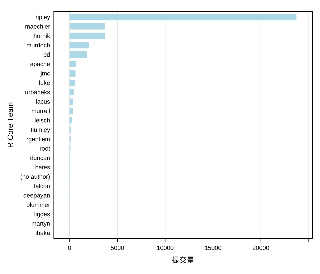
图 3.1: R Core Team 代码提交量的分布

图中 root、(no author) 和 apache 一看就不是正常的人名，请读者忽略。SVN 日志中涉及了部分 R Core Team 成员，笔者将 SVN ID、姓名、主页，整理成表3.1，方便对号入座，这大都是非常低调的一群人。

表 3.1: 2003-2012 年 GNU R 维护者（部分）
SVN ID	姓名	主页
ripley	Brian Ripley	https://www.stats.ox.ac.uk/~ripley/
maechler	Martin Maechler	https://people.math.ethz.ch/~maechler/
hornik	Kurt Hornik	https://statmath.wu.ac.at/~hornik/
murdoch	Duncan Murdoch	https://www.uwo.ca/stats/people/bios/duncan-murdoch.html
pd	Peter Dalgaard	http://staff.pubhealth.ku.dk/~pd/
jmc	John Chambers	https://statweb.stanford.edu/~jmc4/
luke	Luke Tierney	https://homepage.divms.uiowa.edu/~luke/
urbaneks	Simon Urbanek	https://github.com/s-u
iacus	Stefano Iacus	https://github.com/siacus
murrell	Paul Murrell	https://github.com/pmur002
leisch	Friedrich Leisch	https://boku.ac.at/rali/stat/personen/friedrich-leisch
tlumley	Thomas Lumley	https://github.com/tslumley
rgentlem	Robert Gentleman	https://github.com/rgentlem
duncan	Duncan Temple Lang	https://github.com/duncantl
bates	Douglas Bates	https://www.stat.wisc.edu/~bates/
falcon	Seth Falcon	https://github.com/seth
deepayan	Deepayan Sarkar	https://deepayan.github.io/
plummer	Martyn Plummer	https://warwick.ac.uk/fac/sci/statistics/staff/academic-research/plummer/
ligges	Uwe Ligges	https://www.statistik.tu-dortmund.de/ligges.html
martyn	Martyn Plummer	https://warwick.ac.uk/fac/sci/statistics/staff/academic-research/plummer/
ihaka	Ross Ihaka	https://www.stat.auckland.ac.nz/~ihaka/

Martyn Plummer 维护 JAGS 以及 rjags 包
Paul Murrell 维护 grid 包
Douglas Bates 维护 nlme 包
Deepayan Sarkar 维护 lattice 包
……

他们还在 Bioconductor、R Journal、Use R! 和 Journal of Statistical Software 等组织中做了大量工作。

3.1.2 提交量趋势（星期）

接下里，看看每个贡献者提交量的星期分布。Ripley 大人，不管周末还是不周末都会提交大量代码，只是提交量在周六、周日明显要少一些，毕竟也是要休息的。Hornik 和 Ripley 类似，周六日会休息一下，Maechler 在周日休息，Murdoch 没有明显的休息规律，工作日和周末差不多。

# 按星期分组计数
aggr_meta_week <- aggregate(
  x = commit_id ~ contributor + weekday,
  data = spread_meta_data, FUN = function(x) length(unique(x))
)
# 条形图
barchart(
  data = aggr_meta_week, weekday ~ commit_id | contributor, 
  subset = !contributor %in% c("root", "apache", "(no author)"),
  horiz = T, xlab = "提交次数", ylab = "星期几",
  col = "lightblue", border = NA, origin = 0
)

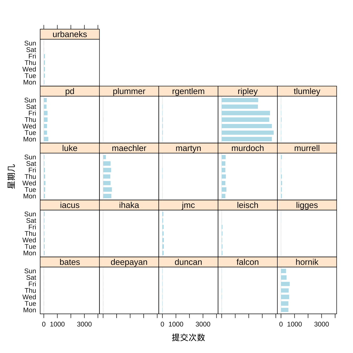
图 3.2: 提交次数的星期分布

接下来看看这 10 年每个贡献者的提交量趋势。

# 分组计数
aggr_meta_ctb_year <- aggregate(
  x = commit_id ~ contributor + year,
  data = spread_meta_data, 
  subset = !contributor %in% c("root", "apache", "(no author)"),
  FUN = function(x) length(unique(x))
)
# 查看数据
head(aggr_meta_ctb_year)

##   contributor year commit_id
## 1          pd 2002         1
## 2       bates 2003        37
## 3      duncan 2003        15
## 4      hornik 2003       785
## 5       iacus 2003       205
## 6       ihaka 2003         5

xyplot(commit_id ~ as.integer(year) | contributor,
  data = aggr_meta_ctb_year,
  subset = !contributor %in% c("root", "apache", "(no author)"),
  type = "b", xlab = "年份", ylab = "提交量", col = "lightblue", pch = 19
)

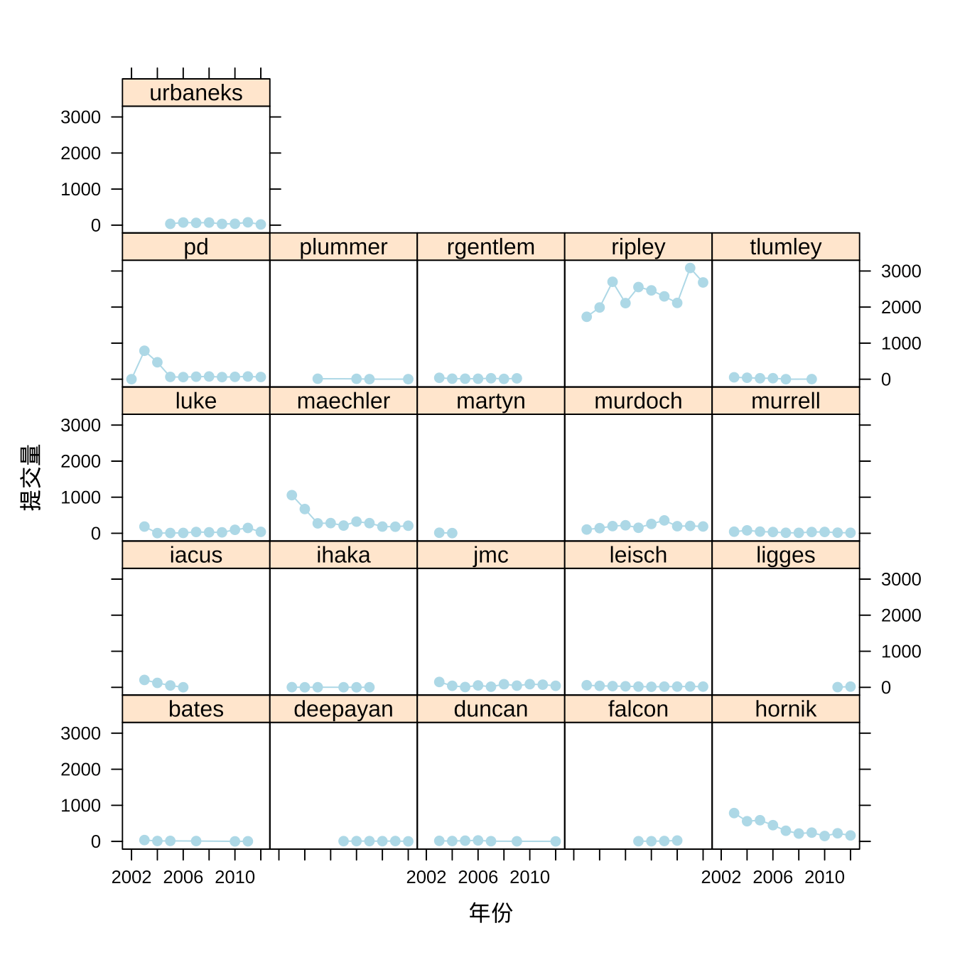
图 3.3: 贡献者年度提交量趋势

原来 R 语言的创始人 Robert Gentleman 和 Ross Ihaka 早就不参与贡献 R Core 代码了。Stefano Iacus、 Martyn Plummer 和 Thomas Lumley 陆续也不活跃了，同时又有 Simon Urbanek、Deepayan Sarkar 和 Uwe Ligges 陆续加入。Ripley 大人在提交量上是如此地遥遥领先，不由得单独进行一波分析。

3.2 Ripley 大人

3.2.1 提交量分布（箱线图）

先按年分组，再按天统计 Ripley 大人的提交量，一年 365 天的提交量分布，如图3.4 所示。

# 按天聚合提交量，保留天所在年、月信息
aggr_meta_day <- aggregate(
  x = commit_id ~ days + month + year, subset = contributor == "ripley",
  data = spread_meta_data, FUN = function(x) length(unique(x))
)
# 查看数据
head(aggr_meta_day)

##   days month year commit_id
## 1    1    01 2003         9
## 2    2    01 2003        10
## 3    3    01 2003         3
## 4    4    01 2003         6
## 5    6    01 2003         2
## 6    8    01 2003         9

Ripley 大人有的时候一天提交 30 多次代码，连续 10 年相当稳定地输出。

bwplot(commit_id ~ year,
  data = aggr_meta_day,
  xlab = "年份", ylab = "提交次数",
  par.settings = list(
    plot.symbol = list(col = "lightblue"),
    box.rectangle = list(col = "lightblue"),
    box.dot = list(col = "lightblue"),
    box.umbrella = list(col = "lightblue")
  )
)

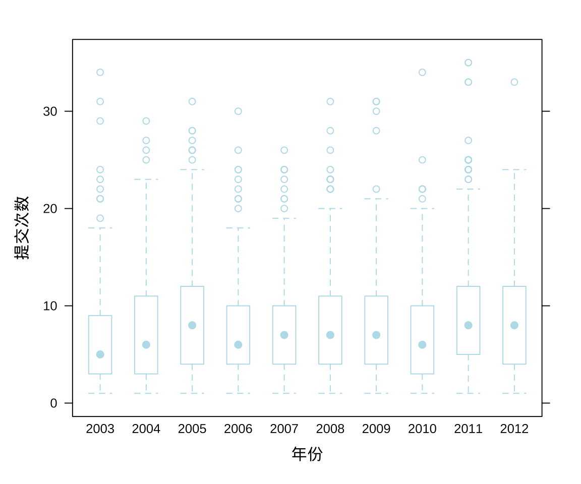
图 3.4: Ripley 大人提交量的分布

3.2.2 提交量分布（提琴图）

相比于葙线图，提琴图可以更加精细地刻画数据的分布，除了5个分位点，它用密度估计曲线描述数据的分布。

bwplot(commit_id ~ year,
  data = aggr_meta_day,
  xlab = "年份", ylab = "提交次数",
  col = 'lightblue', border = NA,
  panel = panel.violin
)

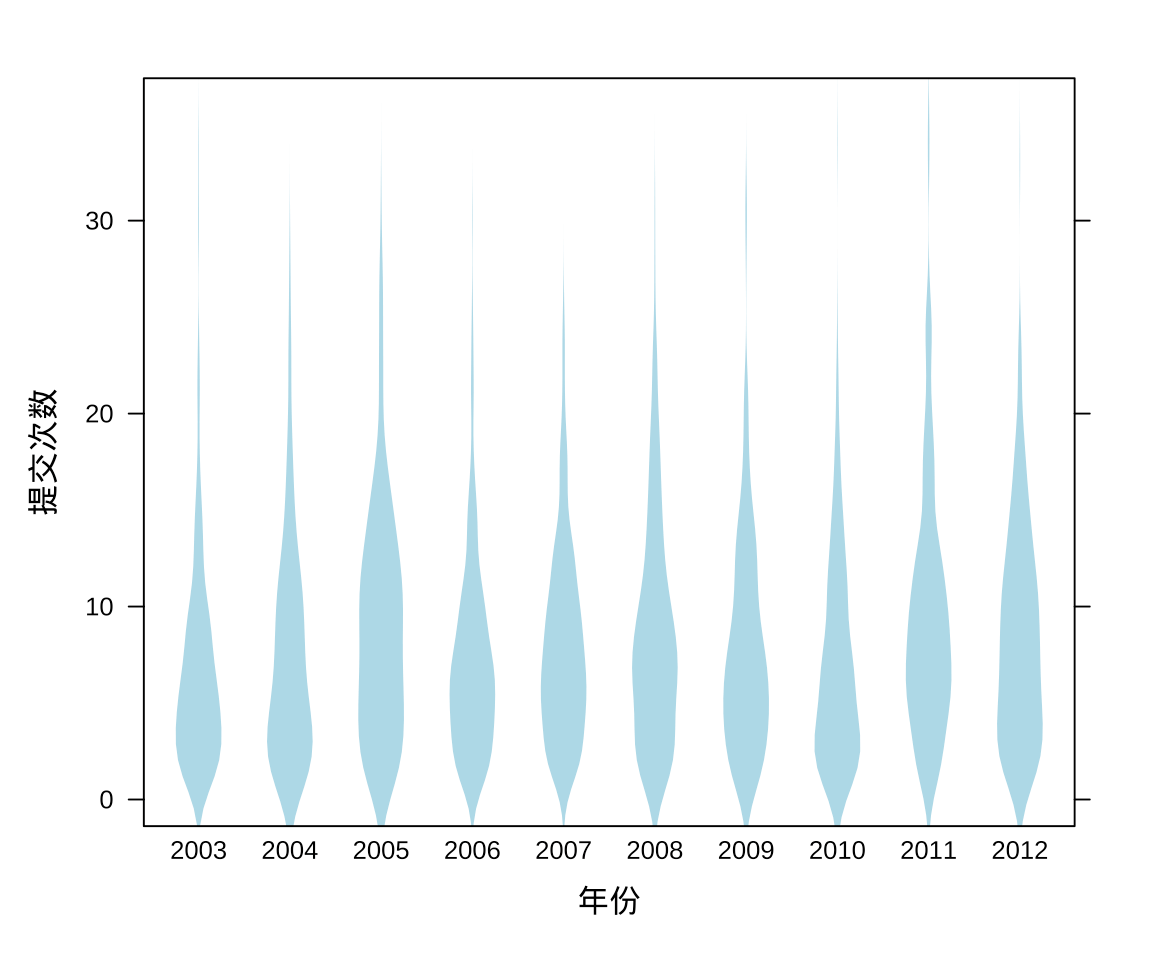
图 3.5: Ripley 大人提交量的分布

3.2.3 提交量分布（密度图）

按年分组，将提交量的分布情况用密度曲线图表示，图中虚线表示提交量的中位数。无论是从提交量的整体分布还是提交量的中位数（可将中位数看作是 Ripley 大人的日平均提交量），Ripley 也是相当稳定地输出呀！

densityplot(~commit_id |  year,
  data = aggr_meta_day, col = 'lightblue', 
  panel = function(x, ...) {
    panel.densityplot(x, plot.points = FALSE,...)
    panel.rug(x, y = rep(0, length(x)), ...)
    panel.abline(v = quantile(x, .5), col.line = "lightblue", lty = 2, lwd = 1.5)
  },
  xlab = "提交次数", ylab = "密度"
)

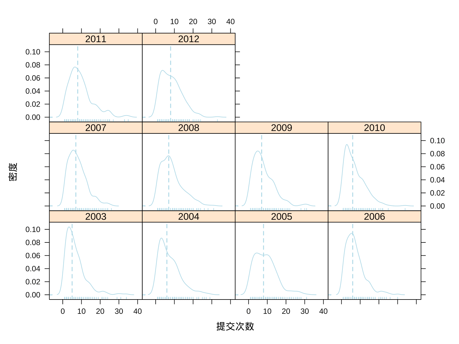
图 3.6: Ripley 大人提交量的分布

3.2.4 提交量趋势（每年）

接下来，看看 Ripley 大人提交量的年度变化趋势。

# 按年统计提交量
aggr_meta_year <- aggregate(
  x = commit_id ~ year,
  data = aggr_meta_day, 
  FUN = sum
)
# 查看数据
head(aggr_meta_year)

##   year commit_id
## 1 2003      1731
## 2 2004      1989
## 3 2005      2701
## 4 2006      2110
## 5 2007      2555
## 6 2008      2463

整体上，看起来提交量在逐年稳定地增加。

xyplot(commit_id ~ as.integer(year), data = aggr_meta_year,
  type = "b", xlab = "年份", ylab = "提交量", col = 'lightblue', pch = 19
)

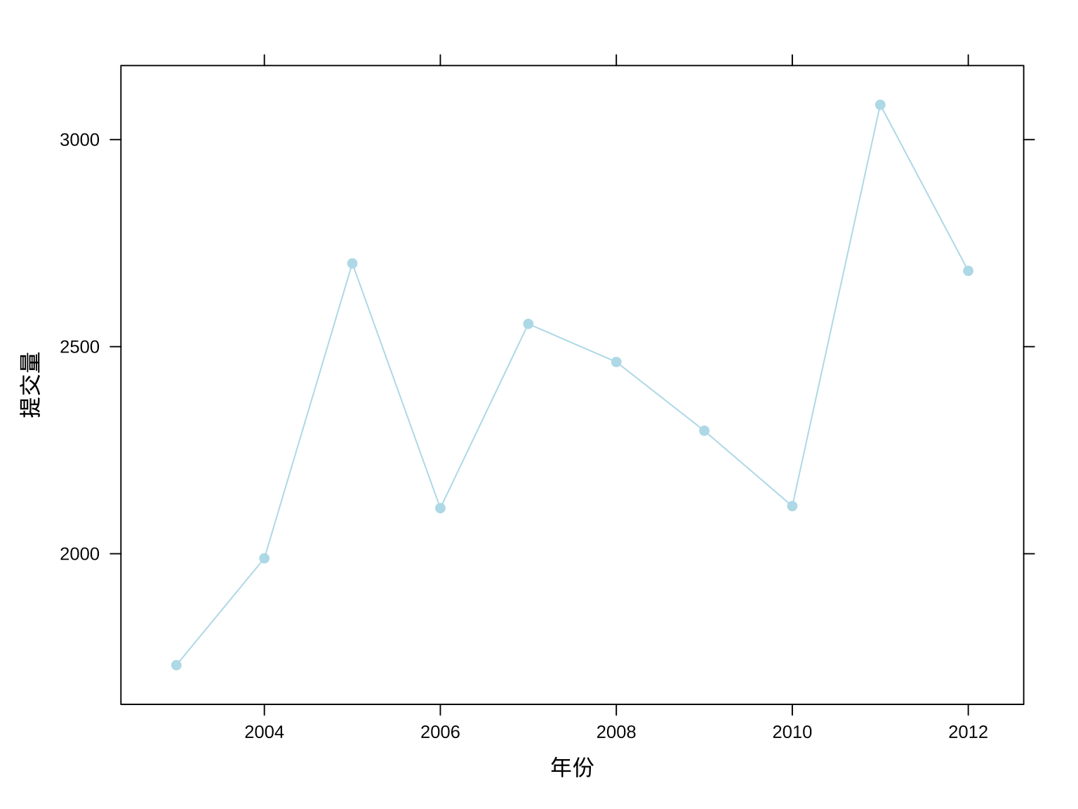
图 3.7: Ripley 大人每年的提交量趋势

3.2.5 提交量趋势（每月）

细分月份来看，Ripley 大人逐年月度提交量趋势。

# 按月统计提交量
aggr_meta_month <- aggregate(
  x = commit_id ~ month + year,
  data = aggr_meta_day, 
  FUN = sum
)
# 查看数据
head(aggr_meta_month)

##   month year commit_id
## 1    01 2003       149
## 2    02 2003       235
## 3    03 2003       152
## 4    04 2003        50
## 5    05 2003       177
## 6    06 2003       177

xyplot(commit_id ~ as.integer(month),
  groups = factor(year), data = aggr_meta_month,
  auto.key = list(columns = 4, space = "top", points = TRUE, lines = TRUE),
  type = c("b", "g"), xlab = "月份", ylab = "提交量", scales = "free",
  lattice.options = list(
    layout.heights = list(
      bottom.padding = list(x = -.1, units = "inches")
    )
  ),
  par.settings = list(
    superpose.line = list(
      lwd = 1.5,
      col = RColorBrewer::brewer.pal(name = "Set3", n = 10)
    ),
    superpose.symbol = list(
      cex = 1, pch = 19,
      col = RColorBrewer::brewer.pal(name = "Set3", n = 10)
    )
  )
)

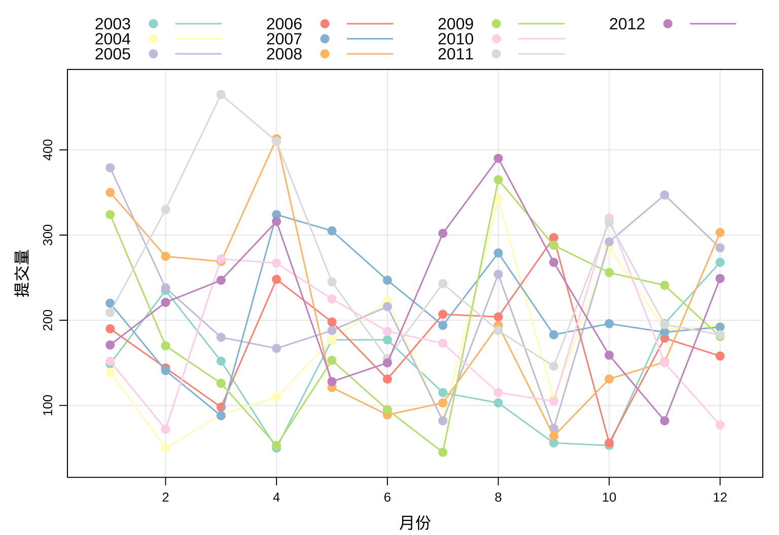
图 3.8: Ripley 大人每月的提交量趋势

看似毫无规律，每年的趋势混合在一起，却正说明 Ripley 大人每年提交代码的量很稳定，很规律。

下面将此数据看作时间序列数据。

aggr_meta_month_ts <- ts(
  data = aggr_meta_month$commit_id, 
  start = c(2003, 1), end = c(2012, 12), 
  frequency = 12, 
  class = "ts", names = "commit_id"
)
aggr_meta_month_ts

##      Jan Feb Mar Apr May Jun Jul Aug Sep Oct Nov Dec
## 2003 149 235 152  50 177 177 115 103  56  53 196 268
## 2004 139  50  89 110 177 223  83 342 108 285 190 193
## 2005 379 238 180 167 188 216  82 254  73 292 347 285
## 2006 190 144  98 248 198 131 207 204 297  56 179 158
## 2007 220 141  88 324 305 247 194 279 183 196 186 192
## 2008 350 275 269 413 121  89 103 194  64 131 151 303
## 2009 324 170 126  53 153  95  45 365 288 256 241 181
## 2010 152  72 272 267 225 187 173 115 105 320 150  77
## 2011 209 330 465 410 245 155 243 188 146 315 195 183
## 2012 171 221 247 316 128 150 302 390 268 159  82 249

以时序图观察 Ripley 大人每月的提交量趋势，如图3.9所示，是不是看起来很平稳呀？那究竟是不是平稳的时间序列呢？

xyplot(aggr_meta_month_ts)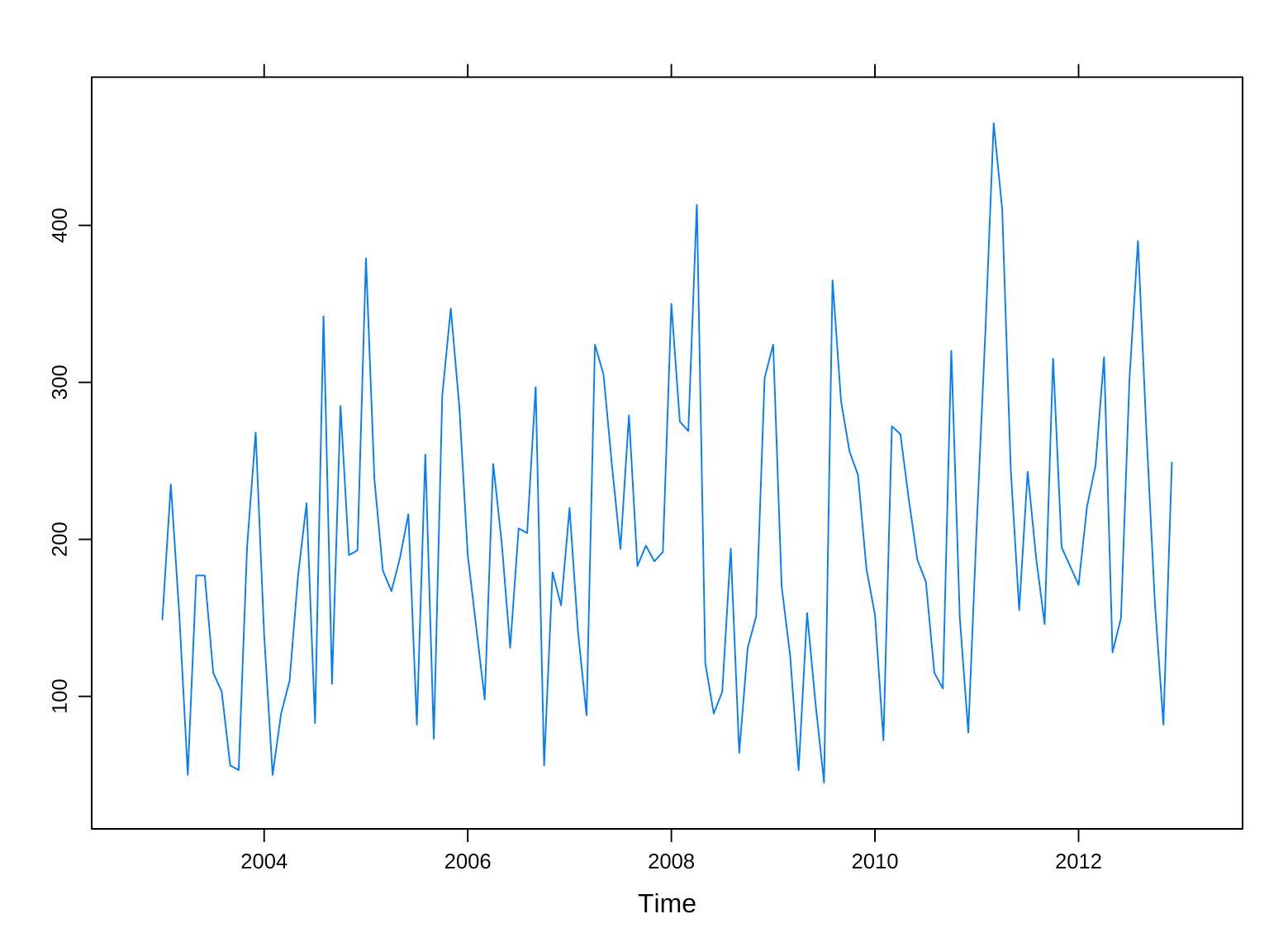

图 3.9: ripley 大人每月的提交量趋势

下面使用 Ljung-Box 检验一下，它的原假设是时间序列是白噪声。

Box.test(aggr_meta_month_ts, lag = 1, type = "Ljung-Box")

## 
##  Box-Ljung test
## 
## data:  aggr_meta_month_ts
## X-squared = 8, df = 1, p-value = 0.005

可见，P 值显著小于 0.05，时间序列不是统计意义上的白噪声，还包含些确定性的信息。

观察时间序列数据中的变化趋势，还可以用水平图，假定 Ripley 大人设定每月提交 100 次代码的 OKR，图3.10可以非常直观地看出每年的完成情况。

library(latticeExtra)
# origin 为基线值，后续值相对于它的增减变化
horizonplot(aggr_meta_month_ts, 
  panel = function(x, ...) {
    latticeExtra::panel.horizonplot(x, ...)
    grid::grid.text(round(x[1]), x = 0, just = "left")
  },
  xlab = "", ylab = "",
  cut = list(n = 10, overlap = 0), # 10 年
  scales = list(draw = FALSE, y = list(relation = "same")),
  origin = 100, 
  colorkey = TRUE, # 右侧梯度颜色条
  col.regions = RColorBrewer::brewer.pal(6, "RdBu"),
  strip.left = FALSE,
  layout = c(1, 10) # 布局 1 列 10 行，每年一行
)

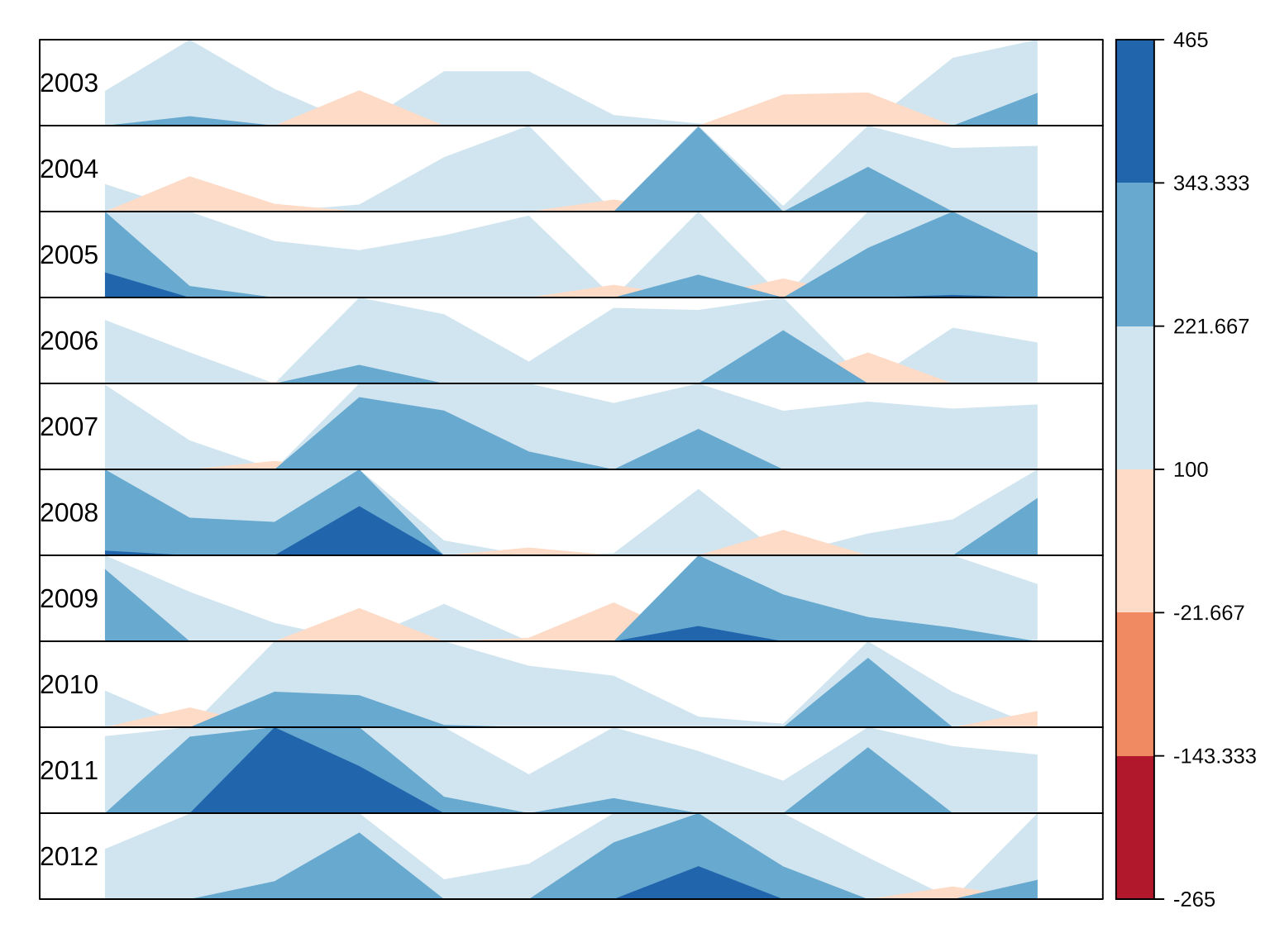
图 3.10: Ripley 大人每月的提交量趋势

3.2.6 提交量趋势（每天）

接下来，再分年按天统计提交量，分组观察趋势变化，如图3.11所示。这就很难看出一些规律了，毕竟每天是否写代码，写多少的影响因素太多，Ripley 大人就是再规律，也不至于规律到每天都一样，或者保持某种明显的趋势。

xyplot(commit_id ~ days | year, data = aggr_meta_day, 
       type = "l", xlab = "天", ylab = "提交量", col = "lightblue")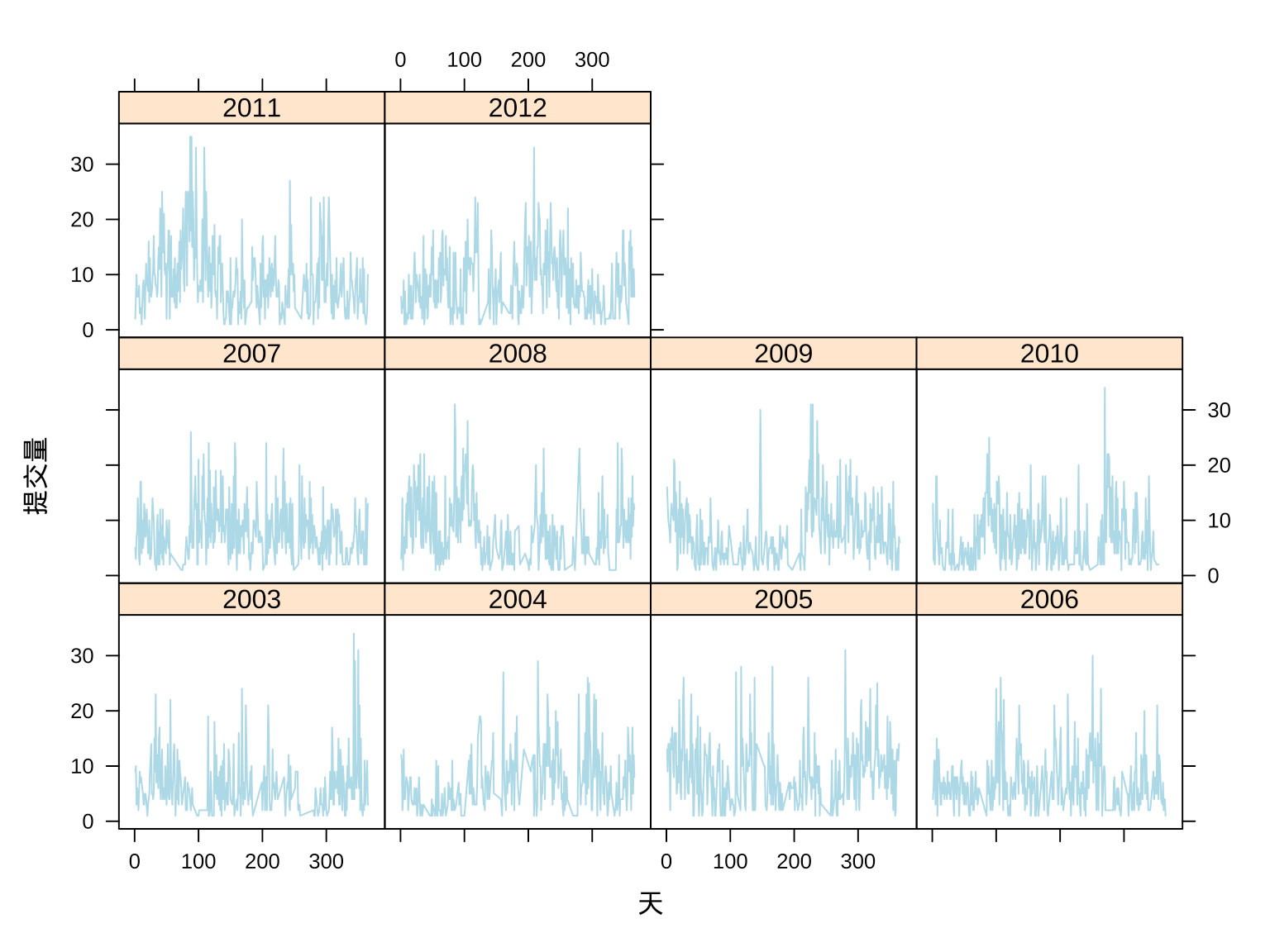

图 3.11: Ripley 大人每天的提交量趋势

3.2.7 提交量趋势（每时）

因此，接下来，按年分组，将每天划分为24个时段，再按时段聚合提交量，就可获得年度提交量分时段的分布，如图3.12所示。将一年 365 天的数据聚合在一块，这就相当地有规律了，规律体现在每天的作息。

# 按年分组，按小时聚合统计
aggr_meta_hour <- aggregate(
  x = commit_id ~ hour + year, subset = contributor == "ripley",
  data = spread_meta_data, FUN = function(x) length(unique(x))
)
# 查看数据
head(aggr_meta_hour)

##   hour year commit_id
## 1    0 2003        13
## 2    1 2003        28
## 3    2 2003        99
## 4    3 2003       186
## 5    4 2003       154
## 6    5 2003       124

每天凌晨 2:00 - 5:00 之间为 Ripley 大人提交量的高峰期，Ripley 大人生活在英国，而英国伦敦和中国北京的时差为 7 小时，也就是说图中凌晨 3:00 - 3:59 相当于北京时间上午 10:00 - 10:59。

xyplot(commit_id ~ hour | year, type = "b", data = aggr_meta_hour, 
       xlab = "时段", ylab = "提交量", col = "lightblue", pch = 19)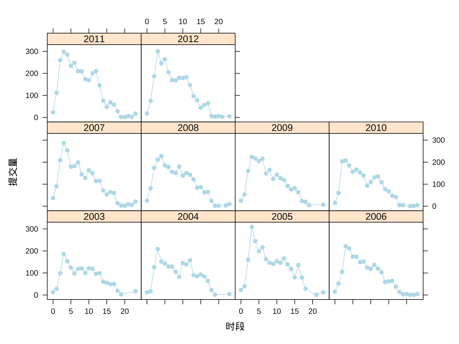

图 3.12: Ripley 大人每小时的提交量趋势

一天 24 小时，Ripley 大人有可能出现在任意一个时段。2005、2007、2011 和 2012 年明显又比其他年份提交量更多些。每年提交代码的高峰时段很稳定，均在北京时间上午 10:00 - 10:59。

4 本文小结

下面从数据探索和数据可视化两个方面谈谈。

有的人何以如此这般的犀利？背后都有一番轻易不为人所知的缘由，唯有拨开云雾才能洞悉其因果。2015 年Yihui Xie在《论R码农的自我修养》中提及 Brian Ripley 大人曾经和蔼可亲，言外之意，Ripley 大人现在手握利器对 R 包、开发者做减法。我也曾吐槽 R 语言社区开源但没有充分利用开源的力量，更像是长期雇佣了 Ripley 大人做维护和开发。甚至在本文写作之前仍有此类似想法 — 基于CRAN 团队在 SVN 上提交的10 年日志数据进行分析，试图回答开源社区是不是谁贡献多谁话语权多？但本文写完，这个问题已不重要，我完全体谅 Ripley 大人，希望出现更多像他这样的维护者。2021 年Dirk Eddelbuettel 曾有篇文章 An Ode to Stable Interfaces: R and R Core Deserve So Much Praise 致敬 R 的稳定性，本文也有此意，特意避开 ggplot2 和一众净土包，也立下十年可重复之约，感谢 Ripley 大人为开源社区的贡献。
可视化在数据探查、数据探索、数据展示都有非常重要的作用，不同的任务对可视化的要求是不一样的。探查的目的是了解数据质量，探索是为了揭示数据蕴含的规律，而展示是为了交流数据信息、洞见。探查和探索的潜在过程尽管耗时费力，但一般不会给读者直接看到，所以，很多时候，大家更多关注可视化的过程和结果。更多详细介绍，推荐读者看看 Antony Unwin 的文章《Why is Data Visualization Important? What is Important in Data Visualization? 》[2]。

5 环境信息

在 RStudio IDE 内编辑本文的 R Markdown 源文件，用 blogdown 构建网站，Hugo 渲染 knitr 之后的 Markdown 文件，得益于 blogdown 对 R Markdown 格式的支持，图、表和参考文献的交叉引用非常方便，省了不少文字编辑功夫。文中使用了多个 R 包，为方便复现本文内容，下面列出详细的环境信息：

xfun::session_info(packages = c(
  "rmarkdown", "blogdown", 
  "lattice", "latticeExtra", "RColorBrewer"
), dependencies = FALSE)

## R version 4.2.1 (2022-06-23)
## Platform: x86_64-apple-darwin17.0 (64-bit)
## Running under: macOS Big Sur ... 10.16
## 
## Locale: en_US.UTF-8 / en_US.UTF-8 / en_US.UTF-8 / C / en_US.UTF-8 / en_US.UTF-8
## 
## Package version:
##   blogdown_1.10       lattice_0.20-45     latticeExtra_0.6-30
##   RColorBrewer_1.1-3  rmarkdown_2.14     
## 
## Pandoc version: 2.18
## 
## Hugo version: 0.101.0

6 参考文献

[1]

Sarkar, D. (2008). Lattice: Multivariate data visualization with r. Springer, New York.

[2]

Unwin, A. (2020). Why is data visualization important? What is important in data visualization? Harvard Data Science Review 2.

从那十年看 R 语言的核心的核心：Brian Ripley 大人

黄湘云